Downloaded 221 times
![Numerical Integration
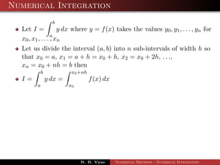
Let I =
b
a
y dx where y = f(x) takes the values y0, y1, . . . , yn for
x0, x1, . . . , xn
Let us divide the interval (a, b) into n sub-intervals of width h so
that x0 = a, x1 = a + h = x0 + h, x2 = x0 + 2h, . . .,
xn = x0 + nh = b then
I =
b
a
y dx =
x0+nh
x0
f(x) dx
Trapezoidal rule:
b=x0+nh
a=x0
f(x)dx =
h
2
[(y0 + yn) + 2 (y1 + y2 + .... + yn)]; h =
b − a
n
If the number of strips is increased; that is, h is decreased, then
the accuracy of the approximation is increased.
N. B. Vyas Numerical Methods - Numerical Integration](https://image.slidesharecdn.com/nm3-120503065749-phpapp01/85/Numerical-Methods-3-5-320.jpg)
![Numerical Integration
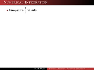
Simpson’s
1
3
rd rule:
x0+nh
x0
f(x)dx = h
3 [(y0 + yn) + 4(y1 + y3 + ....)
+2(y3 + y4 + ....)]; h = b−a
n
N. B. Vyas Numerical Methods - Numerical Integration](https://image.slidesharecdn.com/nm3-120503065749-phpapp01/85/Numerical-Methods-3-7-320.jpg)
![Numerical Integration
Simpson’s
1
3
rd rule:
x0+nh
x0
f(x)dx = h
3 [(y0 + yn) + 4(y1 + y3 + ....)
+2(y3 + y4 + ....)]; h = b−a
n
while applying this rule, the given interval must be divided into
even number of equal sub-intervals. i.e. n must be even.
N. B. Vyas Numerical Methods - Numerical Integration](https://image.slidesharecdn.com/nm3-120503065749-phpapp01/85/Numerical-Methods-3-8-320.jpg)
![Numerical Integration
Simpson’s
1
3
rd rule:
x0+nh
x0
f(x)dx = h
3 [(y0 + yn) + 4(y1 + y3 + ....)
+2(y3 + y4 + ....)]; h = b−a
n
while applying this rule, the given interval must be divided into
even number of equal sub-intervals. i.e. n must be even.
Simpson’s
3
8
th rule:
N. B. Vyas Numerical Methods - Numerical Integration](https://image.slidesharecdn.com/nm3-120503065749-phpapp01/85/Numerical-Methods-3-9-320.jpg)
![Numerical Integration
Simpson’s
1
3
rd rule:
x0+nh
x0
f(x)dx = h
3 [(y0 + yn) + 4(y1 + y3 + ....)
+2(y3 + y4 + ....)]; h = b−a
n
while applying this rule, the given interval must be divided into
even number of equal sub-intervals. i.e. n must be even.
Simpson’s
3
8
th rule:
x0+nh
x0
f(x)dx = 3h
8 [(y0 + yn) + 3(y1 + y2 + y4 + y5 + ....)
+2(y3 + y6 + ....)]; h = b−a
n
N. B. Vyas Numerical Methods - Numerical Integration](https://image.slidesharecdn.com/nm3-120503065749-phpapp01/85/Numerical-Methods-3-10-320.jpg)
![Numerical Integration
Simpson’s
1
3
rd rule:
x0+nh
x0
f(x)dx = h
3 [(y0 + yn) + 4(y1 + y3 + ....)
+2(y3 + y4 + ....)]; h = b−a
n
while applying this rule, the given interval must be divided into
even number of equal sub-intervals. i.e. n must be even.
Simpson’s
3
8
th rule:
x0+nh
x0
f(x)dx = 3h
8 [(y0 + yn) + 3(y1 + y2 + y4 + y5 + ....)
+2(y3 + y6 + ....)]; h = b−a
n
while applying this rule, the number of sub-intervals should be
taken as a multiple of 3 i.e. n must be multiple of 3
N. B. Vyas Numerical Methods - Numerical Integration](https://image.slidesharecdn.com/nm3-120503065749-phpapp01/85/Numerical-Methods-3-11-320.jpg)
![Numerical Integration
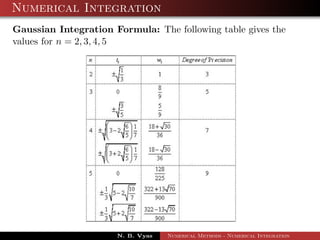
Gaussian Integration Formula:
1
−1
f(t)dt =
n
i=1
wif(ti)
It should be noted here that, t = ±1 is obtained by setting
x =
1
2
[(b + a) + t (b − a)]
N. B. Vyas Numerical Methods - Numerical Integration](https://image.slidesharecdn.com/nm3-120503065749-phpapp01/85/Numerical-Methods-3-12-320.jpg)
![Example
Ex. Evaluate
1
0
e−x2
dx by using Gaussion integration formula for
n = 3.
Sol. Here, we have to first convert the given integral from 0 to 1 into
an integral from −1 to 1. x = 1
2 [(b + a) + t (b − a)], a = 0 and
b = 1
∴ x =
t + 1
2
⇒ dx =
dt
2
∴
1
0
exp(−x2)dx =
1
2
1
−1
exp −
1
4
(t + 1)2 dt
N. B. Vyas Numerical Methods - Numerical Integration](https://image.slidesharecdn.com/nm3-120503065749-phpapp01/85/Numerical-Methods-3-14-320.jpg)
![Error
Error in Quadrature Formula:
If yp is a polynomial representing the function y = f(x) in the
interval [x0, xn] the error in the quadrature formula is given by
E =
xn
x0
f(x) =
xn
x0
ypdx
N. B. Vyas Numerical Methods - Numerical Integration](https://image.slidesharecdn.com/nm3-120503065749-phpapp01/85/Numerical-Methods-3-15-320.jpg)
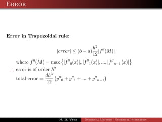
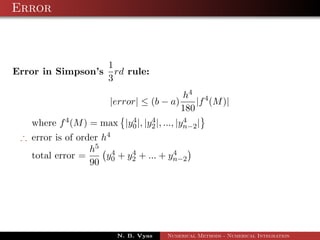
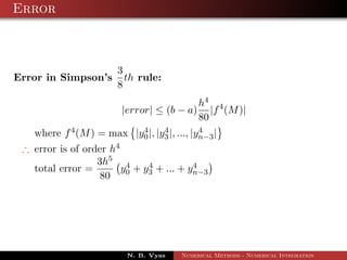

This document discusses numerical integration techniques including the trapezoidal rule, Simpson's 1/3 rule, Simpson's 3/8 rule, and Gaussian integration formulas. It provides the formulas for calculating integration numerically using these methods and notes that accuracy increases with smaller interval widths h. Errors are estimated to be order h^2 for trapezoidal rule and order h^4 for Simpson's rules.