Trend analysis - Lecture Notes

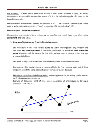
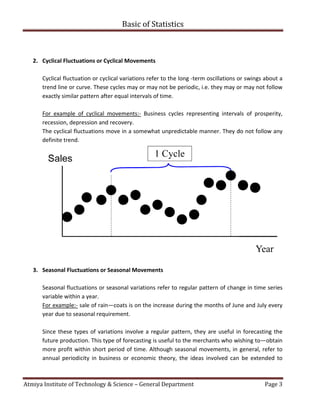
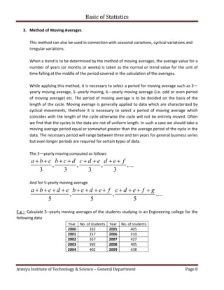
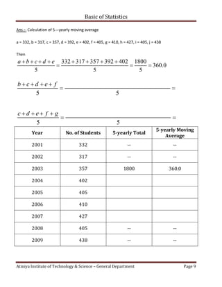
Atmiya Institute of Technology & Science – General Department Page 1
B.E. Sem-IV
Sub: NUMERICAL AND STATISTICAL METHODS FOR COMPUTER ENGINEERING
(2140706)
Topic: Forecasting (Predictions): Trend Analysis
 Introduction
Forecasting is an art of predicting the likelihood of an economic activity or any part thereof for some
future period under certain assumptions or conditions.
When estimates of future conditions are made on a systematic basis, the process is referred to as
‘forecasting’ and the figure or statement obtained is known as a ‘forecast’.
In a world where the future is uncertain, virtually every business and economic decision rests upon
forecast- future conditions. In a modern dynamic world the policy for future has to be necessarily
based on proper vision of the future.
Forecasting aims at reducing the area of uncertainty that surround management decision making
with respect to costs, profit, sales, production, pricing, capital investment and so forth.
“Forecasting refers to the using of knowledge we have at one moment of time to estimate what
will happen at another moment of time. The forecasting problem is created by the interval of time
between the moments."
— Frederick A. Ekeblad
“Forecasting may represent a prediction as to what might happen to one particular item of interest
such as the price of gold next year or in five year's time or it may be prediction as to the future of a
much more complex entity such as the economy or a company."
—.John Argenta
Before we discuss method of forecasting we discuss basic concepts of time series, which is the
foundation for forecasting.
 Time Series
'A time series is a set of chronological observations recorded at successive times or over successive
periods of times. A set of data depending on the time is called time series.’

Atmiya Institute of Technology & Science
For example:- The total annual production of steel
temperatures announced by the weather bureau of a city,
Stock Exchange etc.
Mathematically, a time series is defined by the values
price of a share etc.) at times t1, t2, …. Thus, Y is a function of t, symbolized by Y=F(t).
Classification of Time Series Movements
Characteristic movements of time series may be classified into mainly
components of a time series.
1. Long-term Fluctuations or Trend or Secular Movements
The fluctuations in time series variable due to the factors affecting over a long period of time
are called long-term fluctuations
series. With the trend, the value of the time series variable ten
a long period of time.
The trend or long—term fluctuations represent the general behavior of time series.
For example:- The steady increase in the cost of living by (the consumer price index)
long term period, the trend is towards steady increase or steady decrease.
Example of increasing trend of time series
profit of developing industries
Example of decreasing trend
economy, death-rate, etc.
Basic of Statistics
Atmiya Institute of Technology & Science – General Department
he total annual production of steel in India over a number of years,
by the weather bureau of a city, the daily closing price of a share on the
is defined by the values Y1, Y2, ….., of a variable Y (temperature, closing
, …. Thus, Y is a function of t, symbolized by Y=F(t).
Classification of Time Series Movements
Characteristic movements of time series may be classified into mainly four types
term Fluctuations or Trend or Secular Movements
term fluctuations of the series. Sometimes it is called the trend of the time
. With the trend, the value of the time series variable tends to increase or decrease over
term fluctuations represent the general behavior of time series.
The steady increase in the cost of living by (the consumer price index)
rend is towards steady increase or steady decrease.
of time series:- Increasing population, increasing produ
profit of developing industries etc.
creasing trend of time series:- population of unemployed
Page 2
in India over a number of years, the hourly
the daily closing price of a share on the
, ….., of a variable Y (temperature, closing
four types often called
trend of the time
ds to increase or decrease over
term fluctuations represent the general behavior of time series.
The steady increase in the cost of living by (the consumer price index). For a
Increasing population, increasing production and
loyed in developed

2. Cyclical Fluctuations or Cyclical Movements
Cyclical fluctuation or cyclical variations
trend line or curve. These cycles
exactly similar pattern after equal intervals of time.
For example of cyclical movements
recession, depression and recovery.
The cyclical fluctuations move in a somewhat
definite trend.
3. Seasonal Fluctuations or Seasonal Movements
Seasonal fluctuations or seasonal variations refer to regular pattern of change
variable within a year.
For example:- sale of rain—coats is on the
year due to seasonal requirement.
Since these types of variations involve a regular pattern, they are useful in
future production. This type of forecasting is useful t
more profit within short period of time.
annual periodicity in business or economic theory, the ideas involved can be extended to
Basic of Statistics
yclical Fluctuations or Cyclical Movements
Cyclical fluctuation or cyclical variations refer to the long -term oscillations or swings about a
trend line or curve. These cycles may or may not be periodic, i.e. they may or may not follow
attern after equal intervals of time.
example of cyclical movements:- Business cycles representing intervals of prosperity,
ecession, depression and recovery.
The cyclical fluctuations move in a somewhat unpredictable manner. They do not follow any
Seasonal Fluctuations or Seasonal Movements
Seasonal fluctuations or seasonal variations refer to regular pattern of change
coats is on the increase during the months of June and July every
year due to seasonal requirement.
Since these types of variations involve a regular pattern, they are useful in
future production. This type of forecasting is useful to the merchants who wishing to
more profit within short period of time. Although seasonal movements, in general, refer to
business or economic theory, the ideas involved can be extended to
Page 3
or swings about a
they may or may not follow
cycles representing intervals of prosperity,
do not follow any
Seasonal fluctuations or seasonal variations refer to regular pattern of change in time series
increase during the months of June and July every
Since these types of variations involve a regular pattern, they are useful in forecasting the
who wishing to—obtain
Although seasonal movements, in general, refer to
business or economic theory, the ideas involved can be extended to

include periodicity over any interval
the type of data available.
4. Irregular Fluctuations or Random Movements
The variations in time series variable due to chance
recurring irregular causes are called
For example:- environmental influences, floods, strikes, elections, wars etc.
series data.
Although it is ordinarily assumed that such events produce variations lasting
time, it is conceivable that th
movements.
Time Series Models
The four types of time series components, viz. trend, seasonal, cyclical and
generally interesting in an additive or
overall time series.
If Y is the observed value of time series variable then Y can be represented in symbols as below:
By additive model -> Y = T +
By multiplicative model - > Y = T x S
Where T – Trend Component, C – Cyclical Component, S
Basic of Statistics
periodicity over any interval of time such as hourly, daily, weekly etc. depending
Irregular Fluctuations or Random Movements
The variations in time series variable due to chance, events or random causes
recurring irregular causes are called irregular fluctuations.
environmental influences, floods, strikes, elections, wars etc. influ
Although it is ordinarily assumed that such events produce variations lasting
it is conceivable that they may be so intense as to result in new cyclical or other
The four types of time series components, viz. trend, seasonal, cyclical and irregular
interesting in an additive or multiplicative manner to produce observed values of the
S + C + I
S x C x I
Cyclical Component, S – Seasonal Component, I – Irregular component
Page 4
of time such as hourly, daily, weekly etc. depending on
events or random causes or non—
influence the time
Although it is ordinarily assumed that such events produce variations lasting only a short
in new cyclical or other
irregular fluctuations are
roduce observed values of the
Irregular component

Basic of Statistics
 Measurement of Trend
The various methods that can be used for determining trend are:
1. Freehand or graphic method
2. Semi—average method
3. Moving average method
4. Method of least squares
The method of least squares discussed in previous chapters. First three methods are discussed
below.
1. Freehand or Graphic Method
This is the simplest method of studying trend. The procedure is given below.
1. Plot the time series on a graph.
2. Check the direction of the trend based on the plotted dots.
3. Draw a straight line which best fit to the data according to personal judgment.
Then the line will show the direction of the trend.
A trend line fitted by the freehand method should conform as far as possible following
conditions:
1. It should be smooth i.e. either a straight line or a combination of long gradual curves.
2. The sum of the vertical deviations from the trend of annual observations above the trend
should equal the sum of the vertical deviations from the trend of the observations below
the trend.
3. The sum of the squares of the vertical deviations of the observations from the trend
should be as small as possible.
4. The trend should bisect the cycles so that the area above the trend equals that below the
trend, not only for the entire series but as much as possible for each full cycle.
The fourth condition cannot always be satisfied fully, but attempt should make to observe it
as closely as possible.

Basic of Statistics
E.g.:- Fit a trend line to fit the following data by the freehand method:
Year Production of steel
(million tones)
Year Production of steel
(million tones)
2000 20 2005 25
2001 22 2006 23
2002 24 2007 26
2003 31 2008 25
2004 23
Ans.:- Trend by Free hand method.
Years
The trend line drawn by freehand method can he extended to predict future values.
2. Method of Semi—averages
This method is used, when the given data is divided into two parts, preferably with the same
number of years. For example:- if we are given odd number of years like 7, 11, 15 etc. two
equal parts can be made simply by omitting the middle year.
 After dividing data into two parts, an average (arithmetic mean) of each part is
obtained.
 On the basis of this we get two points.
 Each point is plotted at the mid—point of the class interval covered by the respective
part
Production
(milliontonnes)

Basic of Statistics
 Then the two points are joined by a straight line that gives us the required trend line.
 The line can be extended downwards or upwards in order to get intermediate values
or to predict future values.
E.g.:- Fit a trend line to the following data by the method of semi-averages
Year Sales of Product A
(thousand units)
Year Sales of Product A
(thousand units)
2002 102 2006 108
2003 105 2007 116
2004 114 2008 112
2005 110
Ans.:- Since seven years are given, the middle year shall be left out and an average of the first
three years and the last three years are obtained as follows:
The average of the first three years =
102 105 114 321
107
3 3
 
 
The average of the last three years =
3 3
 
Thus we get two points 107 and __________ which shall be plotted corresponding to their
respective middle years i.e. 2003 and 2007. By joining these points we shall obtain the required trend
line. The actual data and the trend line are shown in the following graph
SalesofProductA
(thousandunits)

Basic of Statistics
3. Method of Moving Averages
This method can also be used in connection with seasonal variations, cyclical variations and
irregular variations.
When a trend is to be determined by the method of moving averages, the average value for a
number of years (or months or weeks) is taken as the normal or trend value for the unit of
time falling at the middle of the period covered in the calculation of the averages.
While applying this method, it is necessary to select a period for moving average such as 3—
yearly moving average, 5--yearly moving, 6—yearly moving average (i.e. odd or even period
of moving average) etc. The period of moving average is to be decided on the basis of the
length of the cycle. Moving average is generally applied to data which are characterized by
cyclical movements, therefore it is necessary to select a period of moving average which
coincides with the length of the cycle otherwise the cycle will not be entirely moved. Often
we find that the cycles in the data are not of uniform length. In such a case we should take a
moving average period equal or somewhat greater than the average period of the cycle in the
data. The necessary period will range between three and ten years for general business series
but even longer periods are required for certain types of data.
The 3—yearly moving computed as follows
, , , ,...
3 3 3 3
a b c b c d c d e d e f       
And for 5-yearly moving average
, , ,...
5 5 5
a b c d e b c d e f c d e f g           
E.g.:- Calculate 5--yearly moving averages of the students studying in an Engineering college for the
following data
Year No. of students Year No. of students
2000 332 2005 405
2001 317 2006 410
2002 357 2007 427
2003 392 2008 405
2004 402 2009 438

Basic of Statistics
Ans.:- Calculation of 5—yearly moving average
a = 332, b = 317, c = 357, d = 392, e = 402, f = 405, g = 410, h = 427, i = 405, j = 438
Then
332 317 357 392 402 1800
360.0
5 5 5
a b c d e       
  
5 5
b c d e f   
 
5 5
c d e f g   
 
Year No. of Students 5-yearly Total
5-yearly Moving
Average
2001 332 -- --
2002 317 -- --
2003 357 1800 360.0
2004 402
2005 405
2006 410
2007 427
2008 405 -- --
2009 438 -- --

Trend analysis - Lecture Notes

More Related Content

What's hot

Similar to Trend analysis - Lecture Notes

More from Dr. Nirav Vyas

Recently uploaded

Trend analysis - Lecture Notes