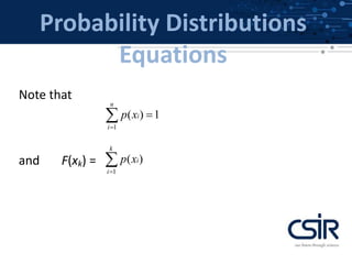
Downloaded 69 times

![Probability Theorems
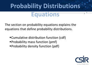
Central Limit Theorem(CLT)
The distribution of the sum of N i.i.d. random
variables becomes increasingly Gaussian as N
grows.
Example: N uniform [0,1] random variables.](https://image.slidesharecdn.com/probabilitydistributionv1-140617024026-phpapp02/85/Probability-distributionv1-23-320.jpg)
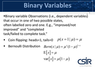
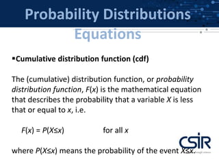
![Binary Variables
N coin flips
Binomial distribution
( | , )p m heads N
0
2
0
( | , ) ( ) (1 )
( | , )
var[ ] ( [ ]) ( | , ) (1 )
m N m
m
N
m
N
m
Bin m N N
m mBin m N N
m m m Bin m N N
](https://image.slidesharecdn.com/probabilitydistributionv1-140617024026-phpapp02/85/Probability-distributionv1-28-320.jpg)
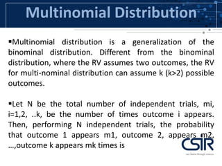
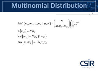
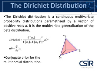


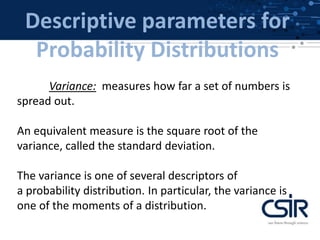
This document provides an overview of probability distributions and related concepts. It defines key probability distributions like the binomial, beta, multinomial, and Dirichlet distributions. It also describes probability distribution equations like the cumulative distribution function and probability density function. Additionally, it outlines descriptive parameters for distributions like mean, variance, skewness and kurtosis. Finally, it briefly discusses probability theorems such as the law of large numbers, central limit theorem, and Bayes' theorem.


![Introduction-to-Probability-Distributions [Autosaved].pptx](https://cdn.slidesharecdn.com/ss_thumbnails/introduction-to-probability-distributionsautosaved-250401053355-25ab20ce-thumbnail.jpg?width=640&height=640&fit=bounds)


