PRESENTED BY
M.PRAVEEN
M.YOGESH
K.VISHAL
S.SURYA
R.VENGATESH
GUIDED BY
ASHOK
(AP/S&H)
SUMMARY
NUMERICAL METHODS IN ENGINEERING
NUMERICAL METHODS IN CRIME DETECTION
NUMERICAL METHODS IN SCIENTIFIC
COMPUTING
NUMERICAL METHODS IN FINDING ROOTS
NUMERICAL METHODS IN HEAT EQUQTION
Introduction
Why are Numerical Methods so widely used in
Engineering?
 Engineers use mathematical modeling (equations and
data) to describe and predict the behavior of systems.
 Closed-form (analytical) solutions are only possible
and complete for simple problems (geometry,
properties, etc.).
 Computers are widely available, powerful, and
(relatively) cheap.
 Powerful software packages are available (special or
general purpose).
A few applications of Numerical Methods in
Engineering:
• Structural/mechanical analysis, design, and
behavior.
• Communication/power
Network simulation
Train and traffic networks
• Computational Fluid Dynamics (CFD):
Weather prediction
Groundwater & pollutant movement
Numerical Methods in Engineering
Topic 1
Overview of the Modelling Process
Why numerical modelling?
To reduce the number of prototypes
constructed.
To use as the forward solver in an
optimization routine to gain the best
possible design.
What are the alternatives?
Design and build lots of physical models
Time consuming
Expensive
Measurement difficulties (cables, calibration,
mechanical precision, interference, mutual coupling,
field confinement, etc)
Analytical solutions
Limited to simple models because of the computational
complexity
Numerical Modelling Procedure
Select/write your numerical modelling
code.
Find a simple analytical model and divide
into segments/pixels/voxels.
These MUST have every dimension less than
l/10 where l is the wavelength in the
material being modelled. (Note that this is
NOT the free space wavelength).
Let’s do the calculation of l
The complex propagation coefficient g is given by the
equation
where
s is the conductivity,
e is the absolute permittivity,
m is the absolute magnetic permeability,
w is the angular radiation frequency, and j is the imaginary number,
a is the attenuation constant
b is the phase constant
)( weswmbag jjj 
The wavelength in the material
b

l
2

At this frequency we have
The wavelength depths on the electromagnetic
properties of the material.
Remember NO segment/pixel/voxel can be larger
than in any dimension l/10 .
This can make life very difficult when you have
electrically large conductive materials.
Solution
MoM and FDTD both use perfectly
conducting materials.
To introduce finite conductivity, we
can use lumped impedance elements.
Maths and crime: Deblurring a
number plate
A short crime story
• Burglar robs a bank
• Escapes in a getaway car
• Pursued by police
GOOD NEWS
Police take a photo
BAD NEWS
Photo is blurred
SOLUTION
Find a model of the blurring process
Blurring function g
Original image
f
• Blurring formula
• Inverting the formula we can get rid the blur
• BUT need to know the blurring function g
ydygyxfxh   2
)()()(

2/)/( 222
dxgdexhdeef xixiyi



Inversion formula
h(x) f(x)
An example of Image
Processing
Scientific computing
Design and analysis of algorithms for
numerically solving mathematical problems
in science and engineering
Considers the effect of approximations and
performs error analysis
modern simulations of engineering
applications
Computational problems:
attack strategy
Develop mathematical model (usually requires a combination of math
skills and some a priori knowledge of the system)
Come up with numerical algorithm (numerical analysis skills)
Implement the algorithm (software skills)
Run, debug, test the software
Visualize the results
Interpret and validate the results
Mathematical modeling
Computational problems:
well-posedness
The problem is well-posed, if
(a) solution exists
(b) it is unique
(c) it depends continuously on problem data
Simplification strategies:
Infinite finite
Nonlinear linear
High-order low-order
What computers can’t do
Solve (by reasoning) general mathematical problems
 they can only repetitively apply arithmetic
primitives to input.
Solve problems exactly.
Represent all numbers. Only a finite subset of the
numbers between 0 and 1 can be represented.
Finding roots / solving equations
General solution exists for equations such as
ax2 + bx + c = 0
The quadratic formula provides a quick answer to all
quadratic equations.
However, no exact general solution (formula) exists
for equations with exponents greater than 4.
Finding roots…
Even if “exact” procedures existed, we are stuck with
the problem that a computer can only represent a
finite number of values… thus, we cannot “validate”
our answer because it will not come out exactly
However we can say how accurate our solution is as
compared to the “exact” solution
Finding roots, continued
Transcendental equations: involving geometric
functions (sin, cos), log, exp. These equations cannot
be reduced to solution of a polynomial.
Convergence: we might imagine a “reasonable”
procedure for finding solutions, but can we guarantee
it terminates?
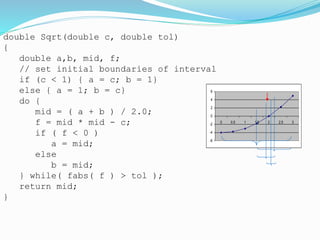
Square root program
If the input c < 1, the root lies between c and 1.
Else, the root lies between 1 and c.
The (positive) square root function is continuous
and has a single solution.
c = x2
F(x) = x2 - c
Example:
F(x) = x2 - 4
-6
-4
-2
0
2
4
6
0 0.5 1 1.5 2 2.5 3
double Sqrt(double c, double tol)
{
double a,b, mid, f;
// set initial boundaries of interval
if (c < 1) { a = c; b = 1}
else { a = 1; b = c}
do {
mid = ( a + b ) / 2.0;
f = mid * mid - c;
if ( f < 0 )
a = mid;
else
b = mid;
} while( fabs( f ) > tol );
return mid;
}
-6
-4
-2
0
2
4
6
0 0.5 1 1.5 2 2.5 3
Heat equations
The heat capacity c of a material gives the amount of
energy needed to raise the temperature T one
kilogram of the material by one degree K (Kelvin).
The thermal conductivity k of a material indicates the
amount
of energy transmitted trough a plate with thickness 1
m and 1sq.m area if the temperatures at the two sides
differ by 1 K.
A(x) ρ c (∂ T (t, x)/∂t)=∂/∂x(k A(x)(∂T (t, x)/∂x))+A(x)f(t,x)
The flux of thermal energy is a vector indicates the
direction of the flow and the amount of thermal
energy flowing per second and square meter
Fourier’s law of heat conduction can be stated as
= −k ∇T
One Dimensional Heat Equation
If a temperature T over a solid (with constant cross
section A) is known to depend on one coordinate x
only, then the change of temperature ∆T measured
over a distance ∆x will lead to a flow of thermal energy
∆Q.
If the time difference is ∆t then
∆Q/∆t = −k A (∆T/∆x)
Two Dimensional Heat Equation
If the domain G ⊂ R2 with boundary curve C describes
a thin plate with constant thickness h then we may
assume that the temperature will depend on t, x and y
only and not on z.
E (t) =
APPLICATION OF NUMERICAL METHODS IN SMALL SIZE

APPLICATION OF NUMERICAL METHODS IN SMALL SIZE

  • 1.
  • 2.
    SUMMARY NUMERICAL METHODS INENGINEERING NUMERICAL METHODS IN CRIME DETECTION NUMERICAL METHODS IN SCIENTIFIC COMPUTING NUMERICAL METHODS IN FINDING ROOTS NUMERICAL METHODS IN HEAT EQUQTION
  • 3.
    Introduction Why are NumericalMethods so widely used in Engineering?  Engineers use mathematical modeling (equations and data) to describe and predict the behavior of systems.  Closed-form (analytical) solutions are only possible and complete for simple problems (geometry, properties, etc.).  Computers are widely available, powerful, and (relatively) cheap.  Powerful software packages are available (special or general purpose).
  • 4.
    A few applicationsof Numerical Methods in Engineering: • Structural/mechanical analysis, design, and behavior. • Communication/power Network simulation Train and traffic networks • Computational Fluid Dynamics (CFD): Weather prediction Groundwater & pollutant movement
  • 5.
  • 6.
    Topic 1 Overview ofthe Modelling Process
  • 7.
    Why numerical modelling? Toreduce the number of prototypes constructed. To use as the forward solver in an optimization routine to gain the best possible design.
  • 8.
    What are thealternatives? Design and build lots of physical models Time consuming Expensive Measurement difficulties (cables, calibration, mechanical precision, interference, mutual coupling, field confinement, etc) Analytical solutions Limited to simple models because of the computational complexity
  • 9.
    Numerical Modelling Procedure Select/writeyour numerical modelling code. Find a simple analytical model and divide into segments/pixels/voxels. These MUST have every dimension less than l/10 where l is the wavelength in the material being modelled. (Note that this is NOT the free space wavelength).
  • 10.
    Let’s do thecalculation of l The complex propagation coefficient g is given by the equation where s is the conductivity, e is the absolute permittivity, m is the absolute magnetic permeability, w is the angular radiation frequency, and j is the imaginary number, a is the attenuation constant b is the phase constant )( weswmbag jjj 
  • 11.
    The wavelength inthe material b  l 2  At this frequency we have The wavelength depths on the electromagnetic properties of the material. Remember NO segment/pixel/voxel can be larger than in any dimension l/10 . This can make life very difficult when you have electrically large conductive materials.
  • 12.
    Solution MoM and FDTDboth use perfectly conducting materials. To introduce finite conductivity, we can use lumped impedance elements.
  • 13.
    Maths and crime:Deblurring a number plate A short crime story • Burglar robs a bank • Escapes in a getaway car • Pursued by police
  • 14.
    GOOD NEWS Police takea photo BAD NEWS Photo is blurred
  • 15.
    SOLUTION Find a modelof the blurring process Blurring function g Original image f • Blurring formula • Inverting the formula we can get rid the blur • BUT need to know the blurring function g ydygyxfxh   2 )()()(
  • 16.
  • 17.
    Scientific computing Design andanalysis of algorithms for numerically solving mathematical problems in science and engineering Considers the effect of approximations and performs error analysis modern simulations of engineering applications
  • 18.
    Computational problems: attack strategy Developmathematical model (usually requires a combination of math skills and some a priori knowledge of the system) Come up with numerical algorithm (numerical analysis skills) Implement the algorithm (software skills) Run, debug, test the software Visualize the results Interpret and validate the results Mathematical modeling
  • 19.
    Computational problems: well-posedness The problemis well-posed, if (a) solution exists (b) it is unique (c) it depends continuously on problem data Simplification strategies: Infinite finite Nonlinear linear High-order low-order
  • 20.
    What computers can’tdo Solve (by reasoning) general mathematical problems  they can only repetitively apply arithmetic primitives to input. Solve problems exactly. Represent all numbers. Only a finite subset of the numbers between 0 and 1 can be represented.
  • 21.
    Finding roots /solving equations General solution exists for equations such as ax2 + bx + c = 0 The quadratic formula provides a quick answer to all quadratic equations. However, no exact general solution (formula) exists for equations with exponents greater than 4.
  • 22.
    Finding roots… Even if“exact” procedures existed, we are stuck with the problem that a computer can only represent a finite number of values… thus, we cannot “validate” our answer because it will not come out exactly However we can say how accurate our solution is as compared to the “exact” solution
  • 23.
    Finding roots, continued Transcendentalequations: involving geometric functions (sin, cos), log, exp. These equations cannot be reduced to solution of a polynomial. Convergence: we might imagine a “reasonable” procedure for finding solutions, but can we guarantee it terminates?
  • 24.
    Square root program Ifthe input c < 1, the root lies between c and 1. Else, the root lies between 1 and c. The (positive) square root function is continuous and has a single solution. c = x2 F(x) = x2 - c Example: F(x) = x2 - 4 -6 -4 -2 0 2 4 6 0 0.5 1 1.5 2 2.5 3
  • 25.
    double Sqrt(double c,double tol) { double a,b, mid, f; // set initial boundaries of interval if (c < 1) { a = c; b = 1} else { a = 1; b = c} do { mid = ( a + b ) / 2.0; f = mid * mid - c; if ( f < 0 ) a = mid; else b = mid; } while( fabs( f ) > tol ); return mid; } -6 -4 -2 0 2 4 6 0 0.5 1 1.5 2 2.5 3
  • 26.
    Heat equations The heatcapacity c of a material gives the amount of energy needed to raise the temperature T one kilogram of the material by one degree K (Kelvin). The thermal conductivity k of a material indicates the amount of energy transmitted trough a plate with thickness 1 m and 1sq.m area if the temperatures at the two sides differ by 1 K. A(x) ρ c (∂ T (t, x)/∂t)=∂/∂x(k A(x)(∂T (t, x)/∂x))+A(x)f(t,x)
  • 28.
    The flux ofthermal energy is a vector indicates the direction of the flow and the amount of thermal energy flowing per second and square meter Fourier’s law of heat conduction can be stated as = −k ∇T
  • 29.
    One Dimensional HeatEquation If a temperature T over a solid (with constant cross section A) is known to depend on one coordinate x only, then the change of temperature ∆T measured over a distance ∆x will lead to a flow of thermal energy ∆Q. If the time difference is ∆t then ∆Q/∆t = −k A (∆T/∆x)
  • 30.
    Two Dimensional HeatEquation If the domain G ⊂ R2 with boundary curve C describes a thin plate with constant thickness h then we may assume that the temperature will depend on t, x and y only and not on z. E (t) =

Editor's Notes

  • #18 George Mason University, Department of Mathematical Sciences
  • #19 George Mason University, Department of Mathematical Sciences
  • #20 George Mason University, Department of Mathematical Sciences