Download as PDF, PPTX
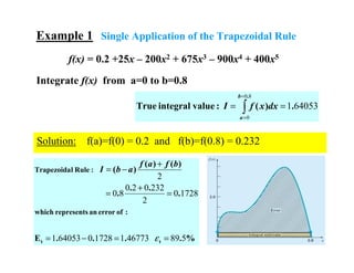
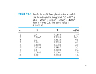

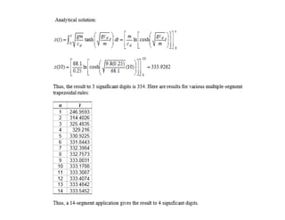
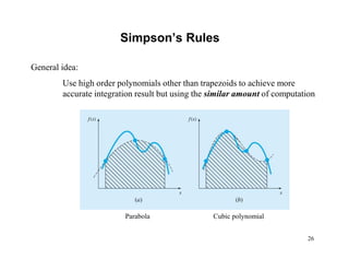
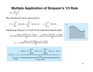
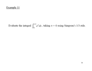
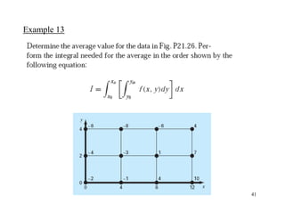
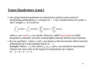
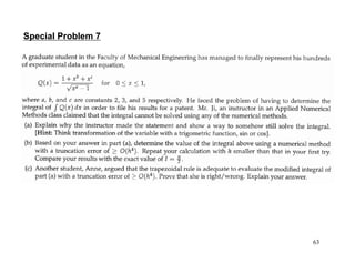
![Solution (cont)
+
++
−
= ∑
−
=
)(f)iha(f)(f
)(
I
i
3028
22
830 12
1
[ ])(f)(f)(f 301928
4
22
++=
[ ]6790175484227177
4
22
.).(. ++=
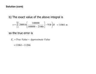
m11266=
Then:](https://image.slidesharecdn.com/appliednumericalmethodslec10-150507042353-lva1-app6892/85/Applied-numerical-methods-lec10-15-320.jpg)
![)()(
)(
)(
2
2
1
212
2
2
1
2
1
≅⇒≅
h
h
hEhE
h
h
hE
hE
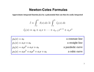
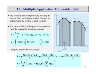
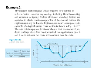
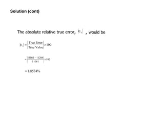
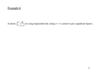
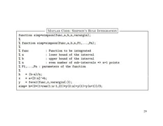
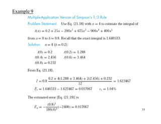
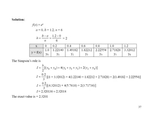
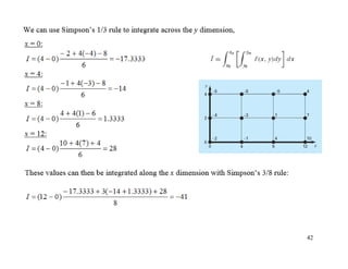
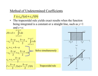
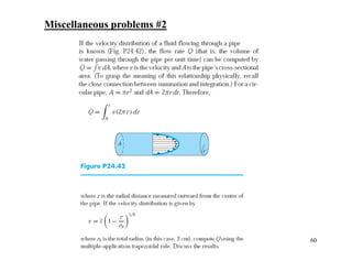
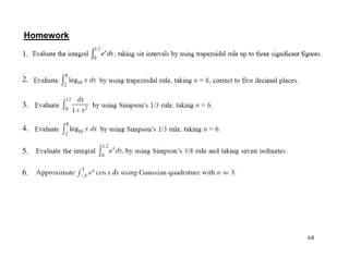
Romberg Integration
Successive application of the trapezoidal rule to attain efficient numerical integrals of functions.
Richardson’s Extrapolation:
Uses two estimates of an integral to compute a third and more accurate approximation.
sizes)stepdifferentforconstantis(assume
)()()()(
/)(/)()()(
)
2
(
2
12
2211
fhOfh
ab
E
hEhIhEhI
habnnabhhEhII
′′=′′
−
≅
+=+
−=−=+=
I = exact value of integral E(h) = the truncation error
I(h): trapezoidal rule (n segments, step size h)
Improved estimate of the integral.
It is shown that the error of this
estimate is O(h4). Trapezoidal rule
had an error estimate of O(h2).( )
[ ])()(
/
)(
)()(
122
21
2
22
1
1
hIhI
hh
hII
hEhII
−
−
+≅
+=
( )
( ) 1/
)()(
)()()(/)()( 2
21
12
222
2
2121
−
−
≅⇒+≅+
hh
hIhI
hEhEhIhhhEhI](https://image.slidesharecdn.com/appliednumericalmethodslec10-150507042353-lva1-app6892/85/Applied-numerical-methods-lec10-24-320.jpg)
![25
( )
[ ])()(
1/
1
)( 122
21
2 hIhI
hh
hII −
−
+≅
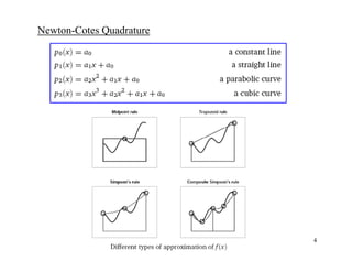
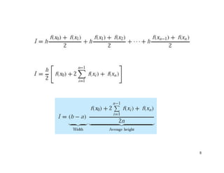
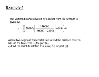
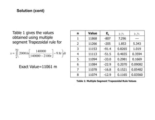
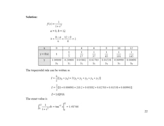
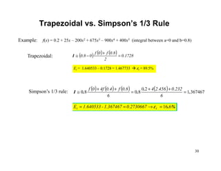
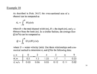
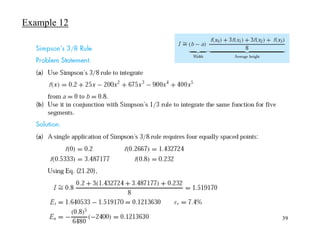
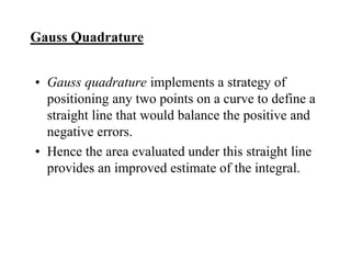
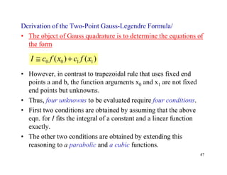
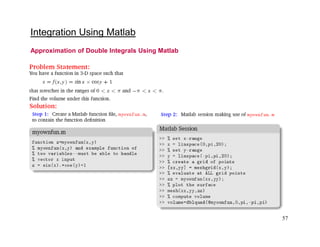
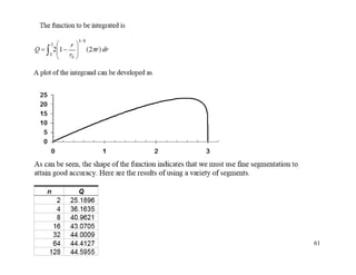
Example 7
Evaluate the integral of f(x) = 0.2 +25x – 200x2 + 675x3 – 900x4 + 400x5
from a=0 to b=0.8. I (True Integral value) = 1.6405
Segments h Integral εtr%
1 0.8 0.1728 89.5
2 0.4 1.0688 34.9
4 0.2 1.4848 9.5
%)6.16(0.2733675.16405.1E
3675.1)1728.0(
3
1
)0688.1(
3
4
:givetocombined2&1Segments
tt ==−=
=−≅
ε
I
In each case, two estimates with
error O(h2) are combined to give a
third estimate with error O(h4)
%)1(0.01716234.16405.1E
6234.1)0688.1(
3
1
)4848.1(
3
4
:givetocombined4&2Segments
tt ==−=
=−≅
ε
I
)2/(If 12 ⇒= hh [ ] )(
3
1
)(
3
4
)()(
12
1
)( 121222 hIhIhIhIhII −=−
−
+≅](https://image.slidesharecdn.com/appliednumericalmethodslec10-150507042353-lva1-app6892/85/Applied-numerical-methods-lec10-25-320.jpg)
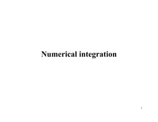
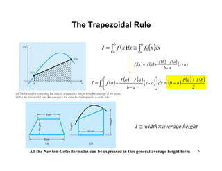
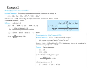
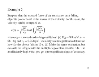
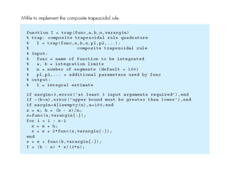
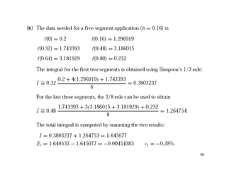
![• More accurate estimate of an integral is obtained if
a high-order polynomial is used to connect the
points. These formulas are called Simpson’s rules.
Simpson’s 1/3 Rule: results when a 2nd order
Lagrange interpolating polynomial is used for f(x)
dxxf
xxxx
xxxx
xf
xxxx
xxxx
xf
xxxx
xxxx
I
dxxfdxxfI
x
x
b
a
b
a
xbxa
xf
∫
∫ ∫
−−
−−
+
−−
−−
+
−−
−−
=
≅=
==
2
0
)(
))((
))((
)(
))((
))((
)(
))((
))((
)()(
2
1202
10
1
2101
20
0
2010
21
20
2
Using
.polynomialorder-secondais)(2where
[ ] RULE1/3SSIMPSON'
2
)()(4)(
3
210
:resultsformulafollowingtheon,manipulatialgebraicandnintegratioafter
⇐
−
=++≅
ab
hxfxfxf
h
I
a=x0 x1 b=x2
Simpson’s Rules](https://image.slidesharecdn.com/appliednumericalmethodslec10-150507042353-lva1-app6892/85/Applied-numerical-methods-lec10-27-320.jpg)
![28
[ ] RULE1/3SSIMPSON'
2
)()(4)(
3
210
:resultsformulafollowingtheon,manipulatialgebraicandnintegratioafter
⇐
−
=++≅
ab
hxfxfxf
h
I](https://image.slidesharecdn.com/appliednumericalmethodslec10-150507042353-lva1-app6892/85/Applied-numerical-methods-lec10-28-320.jpg)
![38
[ ]
8
)()(3)(3)(
)(
)()(3)(3)(
8
3
)()(
3210
3210
3
3
)(
xfxfxfxf
abI
xfxfxfxf
h
I
dxxfdxxfI
ab
h
b
a
b
a
+++
−≅
+++≅
≅=
−
=
∫ ∫
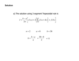
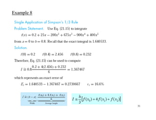
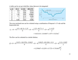
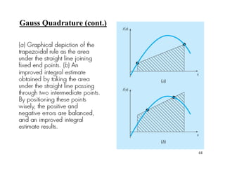
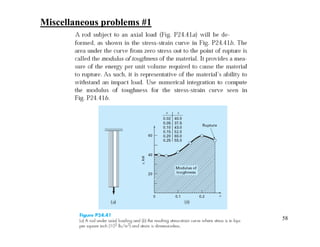
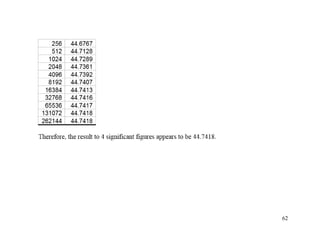
Simpson’s 3/8 Rule
Simpson’s 1/3 and 3/8 rules can be
applied in tandem to handle
multiple applications with odd
number of intervals
Fit a 3rd order Lagrange interpolating
polynomial to four points and integrate](https://image.slidesharecdn.com/appliednumericalmethodslec10-150507042353-lva1-app6892/85/Applied-numerical-methods-lec10-38-320.jpg)
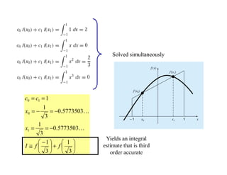
![50
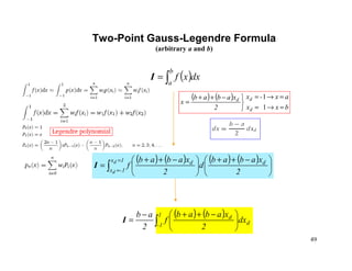
Example of Two-Point Gauss-Legendre Formula
( ) 8225781264592532918525140
3
1
3
1
40 ....ff.I dd =+=
+
−
=
( ) ( )∫∫ +==
1
1-
0.8
0 dd dx0.4x0.4f0.4dxxfI
( )∫=
1
1- ddd dxxf40.I
Example14: f(x) = 0.2 + 25x – 200x2 + 675x3 – 900x4 + 400x5 (integral between a=0 and b=0.8)
x = 0.4 + 0.4xd
dx = 0.4 dxd
( ) ( ) ( ) ( ) ( )[ ]∫ +++−+++−++=
1
1- dddddd dx0.4x0.40.4x0.40.4x0.40.4x0.40.4x0.4250.20.4
543
400900675200 2
I
( ) ( )
bxx
ax-x
2
xabab
x
d
dd
=→=
=→=
−++
=
1
1
)()( 1100 xfcxfcI +≅](https://image.slidesharecdn.com/appliednumericalmethodslec10-150507042353-lva1-app6892/85/Applied-numerical-methods-lec10-50-320.jpg)
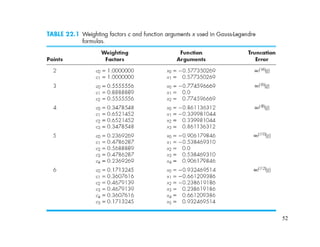
![51
Higher-Point Gauss-Legendre Formula
( ) ( ) ( )[ ]2d21d10d0 xfcxfcxfc ++= 40.I
( ) ( ) ( ) ( )
44444444 344444444 21
L
44444 344444 21
444 3444 21
pointn
1-n1-n
pointthree
22
pointtwo
1100 xfcxfcxfcxfc
−
−
−
++++≅I
( )∫=
1
1- ddd dxxf40.I
Example: f(x) = 0.2 + 25x – 200x2 + 675x3 – 900x4 + 400x5 (integral between a=0 and b=0.8)
Three-point Gauss-Legendre formula: c0 = 0.5555556 x0 = - 0.774596669
c1 = 0.8888889 x1 = 0.0
c2 = 0.5555556 x2 = 0.774596669
( ) ( ) ( )[ ].77459669f0.5555560f0.88888890.77459669-f0.5555560.4 ddd ++=I
1.640533](https://image.slidesharecdn.com/appliednumericalmethodslec10-150507042353-lva1-app6892/85/Applied-numerical-methods-lec10-51-320.jpg)
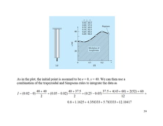

The document discusses numerical integration methods such as Newton-Cotes formulas, the trapezoidal rule, and Simpson's rules. The trapezoidal rule approximates the integral of a function f(x) between bounds a and b by taking the average of f(a) and f(b) and multiplying by the width b-a. Simpson's rules use higher order polynomials to connect function values for a more accurate approximation of the integral. Gauss quadrature implements strategic positioning of points to define straight lines that balance positive and negative errors, improving the integral estimate.