This document discusses various numerical integration techniques including Newton-Cotes formulas, the trapezoidal rule, Simpson's rules, integration with unequal segments, open integration formulas, integration of equations, and Romberg integration. The key Newton-Cotes formulas covered are the trapezoidal rule, Simpson's 1/3 rule, and Simpson's 3/8 rule. The document provides examples of applying these formulas to numerically evaluate definite integrals and calculates the associated errors. It also discusses using Richardson extrapolation, known as Romberg integration, to iteratively improve the accuracy of numerical integration compared to the standard Newton-Cotes formulas.

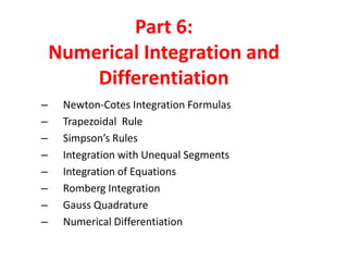
1. Part 6:
Numerical Integration and
Differentiation
–
–
–
–
–
–
–
–
Newton-Cotes Integration Formulas
Trapezoidal Rule
Simpson’s Rules
Integration with Unequal Segments
Integration of Equations
Romberg Integration
Gauss Quadrature
Numerical Differentiation

2. Newton-Cotes Integration Formula
 Replacing the complicated integrand function or tabulated data by
an approximating function such as a polynomial.
f(x)
f(x)
Replacing by a
straight line
x
Replacing by a
parabola
x
 These formulas are applicable to both closed forms (i.e., data points
at the beginning and end of the integration limits are known) and
open forms (otherwise).
 These formulas are applied for equally spaced intervals.

3. Trapezoidal Rule
 Complicated integrand function is
replaced by a first order polynomial
(straight line).
b
I
f(x)
b
f ( x ) dx
a
f 1 ( x ) dx
a
where the first-order polynomial
f1 ( x )
f (a )
f (b )
f (a )
b
b
I
f (a )
f (b )
(b
a
I
(b
a)
a
(x
a)
a
f (a )
(x
a ) dx
a)
f (a )
f (b )
2
Trapezoidal rule
b
x

4. f(x)
f(a)+f(b)
2
=average height
f(a)
I
( width ) ( average
height )
f(b)
b
a
x
width
 All the Newton-Cotes formulas can be formulated in general
form above (only definition of average height changes).
Error for trapezoidal rule:
b
''
f ( x ) dx
Et
1
''
f ( )( b
12
Local truncation error
a)
3
Ea
1
12
(b
3
''
a) f
''
f
a
(b
a)
Average of the second
derivative between the interval

5. EX: Numerically integrate
f ( x)
0 .2
25 x
200 x
2
675 x
3
900 x
4
400 x
5
from a=0 to b=0.8. Find the error. (Note that the exact solution is 1.6405).
f (0)
0 .2
f ( 0 .8 )
Et
I
0 .8
0 .2
0 . 1728
2
0 . 232
1 . 6405
0 . 232
0 . 1728
1 . 4677
t
89 . 5 %
Normally, we don’t have the knowledge of the true error; we can calculate the
approximate error. We need to calculate the second derivative of the function:
''
f ( x)
400
4050 x
10800 x
2
8000 x
3
0 .8
400
''
f
4050 x
10800 x
0
Ea
12
8000 x
3
60
0 .8
1
2
( 60 )( 0 . 8 )
3
0
2 . 56
Et and Ea have the
same order and sign

6. Multiple-application trapezoidal rule:
We can increase the accuracy of the integration by dividing the
interval into many segments and apply the trapezoidal rule to
each segment.
f(x)
For n+1 equally spaced base
points, there are n segments of
step size:
h
(b
a)
n
I
h
2
x0
h
n 1
f ( x0 )
2
f ( xi )
f ( xn )
i 1
Initial point
x1
final point
x2
x

7. or
n 1
f ( x0 )
I
(b
2
f ( xi )
f ( xn )
i 1
a)
2n
width
average height
Error for the multiple-application trapezoidal rule is found by
summing individual errors.
b
Et
a
12 n
or
3
n
''
f ( i)
3
i 1
n
Ea
b
a
12 n
2
''
3
''
f
where
f (
''
f
i 1
n
i
)
Convergence:
Error is inversely
related to the
square of n !

8. EX: Use two-segment trapezoidal rule to integrate
f ( x)
0 .2
2
675 x
f ( 0 .4 )
25 x
2 . 456
200 x
3
900 x
4
400 x
5
From a=0 to b=0.8.
n=2
h=0.4
f (0)
I
0 .8
0 .2
0 .2
2 ( 2 . 456 )
0 . 232
f ( 0 .8 )
0 . 232
1 . 0688
4
Ea
1 . 6405
1
12 ( 2 )
2
( 60 )( 0 . 8 )
3
t
34 . 9 %
0 . 64
Error is inversely
related to the square
of n.
1.0688
34.9
3
1.3695
16.5
1.4848
9.5
5
0 . 57173
I
4
1 . 0688
n
2
Et
1.5399
6.1
6
1.5703
4.3
7
1.5887
3.2
8
1.6008
2.4
t

9. Simpson’s Rules
f(x)
Instead of using a line segment, use
higher-order polynomials to connect
points increase the accuracy.
Simpson’s 1/3 rule
x1
x0
A parabola is substituted for the function.
Lagrange polynomial forms are used for the replacement.
Replacing Lagrange polynomials for the function at three
points x0 , x1, and x2 :
(x
x2
I
x0
x1 )( x
( x0
x2 )
x1 )( x 0
(x
x 0 )( x
( x2
x 0 )( x 2
x2 )
f ( x0 )
x1 )
x1 )
f ( x2 )
(x
x 0 )( x
( x1
x 0 )( x1
x2 )
x2 )
f ( x1 )
dx
x2
x

10. After integration and algebraic manipulations
1h
I
3
f ( x0 )
4 f ( x1 )
f x2
Simpson’s 1/3
rule.
In another form:
I
(b
f ( x0 )
a)
4 f ( x1 )
f x2
h=(b-a)/2
6
width
average height
Error for the single segment Simpon’s 1/3 rule:
Et
(b
a)
2880
5
f
(4)
> It is more accurate than expected as the
error is related to the forth order derivative
(third order term is meaningful but is zero).
> It yields exact results for cubic polynomials
even though it is obtained from a parabola.

11. EX: Use single application of Simpson’s 1/3 rule to integrate
f ( x)
0 .2
2
675 x
f ( 0 .4 )
2 . 456
25 x
200 x
3
900 x
4
400 x
5
from a=0 to b=0.8.
n=2
h=0.4
f (0)
I
0 .8
0 .2
0 .2
4 ( 2 . 456 )
0 . 232
f ( 0 .8 )
0 . 232
1 . 3675
6
Et
1 . 6405
1 . 3675
0 . 273
t
16 . 6 %
0 .8
f
(4)
( x)
21600
f
48000 x
(4)
f
(4)
0
2400
0 .8
Ea
(b
a)
2880
5
(4)
f
( 0 .8 )
2880
5
( 2400 )
( x ) dx
0 . 273
0
Et and Ea are equal
because the integrand is
a fifth order polynomial

12. Multiple-application Simpson’s 1/3 rule
For n segments:
h
(b
a)
n
Total integral can be represented
x2
I
xn
x4
f ( x ) dx
x0
f ( x ) dx
...
x2
f ( x ) dx
xn
2
Substituting Simpson’s 1/3 formula
n 1
f ( x0 )
I
(b
a)
4
n 2
f ( xi )
2
i 1, 3 , 5
f ( xi )
i 2,4,6
3n
width
average height
f ( xn )

13. Error for the multiple (n) segment
Simpon’s 1/3 rule is calculated by
adding error for individual segments.
Hence, we get:
Et
(b
a)
180 n
4
5
(4)
f
Multiple application Simpson’s rule returns very accurate results
compare to trapezoidal rule. It is the method of choice for most
applications.
 As for all Newton-Cotes formulas, the intervals must be equally
spaced.
Because of the need for three points for applications, the method
is limited to odd number of points (even number of segments).

14. EX: Use multiple application Simpson’s 1/3 rule (n=4) to integrate
f ( x)
2
675 x
f ( 0 .2 )
1 . 288
3 . 464
f ( 0 .8 )
0 . 232
3 . 464 )
2 ( 2 . 456 )
0 .2
25 x
200 x
3
900 x
4
400 x
5
from a=0 to b=0.8.
n=4
h=0.2
f (0)
f ( 0 .6 )
I
0 .8
0 .2
4 (1 . 288
0 .2
f ( 0 .4 )
0 . 232
2 . 456
1 . 6235
12
Et
Ea
1 . 640533
1 . 623467
a)
5
180 ( n )
4
(b
(4)
f
0 . 017067
( 0 .8 )
t
1 . 04 %
5
180 ( 4 )
4
( 2400 )
0 . 017067
Small error shows very
accurate results are
obtained.

15. Simpson’s 3/8 rule
Simpson’s 3/8 rule is used when the odd-number of segments
are encountered.
A third-order polynomial is used for replacing the function.
b
I
b
f ( x ) dx
f 3 ( x ) dx
a
a
Applying a third order Legendre polynomial to four points gives
I
3h
f ( x0 )
8
I
(b
a)
3 f ( x1 )
f ( x0 )
3 f ( x2 )
3 f ( x1 )
3 f ( x2 )
8
width
f x3
average height
f x3
Simpson’s 3/8
formula.
h=(b-a)/3

16. Truncation error for Simpson’s 3/8 rule:
Et
(b
a)
5
f
(4)
6480
Simpson’s 3/8 rule is
somewhat more
accurate than 1/3 rule
In general Simpson’s 1/3 rule is the method of choice because of
obtaining third order accuracy and using three points instead of
four.
3/8 rule has the utility when the number of segments is odd.
In practice, use 1/3 rule for all the even number of segments and
use 3/8 rule for the remaining last three segments.
Higher-order Newton-Cotes formulas:
Higher order (n=4,5) formulas have the same order error as n=1
(Trapezoid) or n=2,3 (Simpson’s) formulas.
Higher-order formulas are rarely used in engineering practices.
To increase the accuracy, just increase the number of segments!

17. Integration with Unequal Segments
There may be cases where the spacing between data points may
not be even (e.g., experimentally derived data points)
One way is to use trapezoidal rule for each segment
I
h1
f ( x0 )
f ( x1 )
2
h2
f ( x1 )
f ( x2 )
2
..
hn
f ( xn 1 )
f ( xn )
2
width of the segments (h) are not constant so the
formula cannot be written in a compact form.
A computer algorithm can easily be developed to do the
integration for unequal-sized segments.
The algorithm can be constructed such that, use Simpson’s 1/3
rule wherever two consecutive equal-sized segments are
encountered, and use 3/8 rule wherever three consecutive
equal-sized segments are encountered. When adjacent
segments are unequal-sized , just use trapezoidal rule.

18. Open Integration Formulas
 There may be cases where
integration limits are beyond the
f(x)
range of the data.
General characteristics and order of
error for open forms of the NewtonCotes formulas are similar to the
closed forms.
Even segment formulas are usually
the method of choice as they
require fewer points.
a
b
x
Open forms are not used for definite integration.
They have utility for analyzing improper integrals (discussed later).
They have connection to multi-step method for solving ordinary
differential equations.

19. Integration of Equations
Use of multiple-application of
trapezoidal and Simpson’s rules are
not convenient for analyzing
integration of functions.
> Large number of operations
required to evaluate the functions.
> For large values of n, round of
errors starts to dominate.
Percent relative error
Previously discussed methods are appropriate for tabulated data.
If the function to be integrated is available, other modified
methods are available.
> Romberg integration (Richardson extrapolation)
> Gauss quadrature
Newton-Cotes method for functions:
Trapezoidal
rule
Simpson’s
rule
n

20. Romberg Integration
It uses the trapezoidal rule, but much more efficient results are
obtained through iterative refinement techniques .
Richardson’s extrapolation:
A sequence acceleration method to improve the rate of
convergence.
It offers a very practical tool for numerical integration and
differentiation.
Application of iterative refinement techniques to improve the
error at each iteration. For each iteration
I
exact
integral
I (h)
E (h)
approximate
integral
truncation
error
In Richardson extrapolation, two approximate integrals are used
to compute a third more accurate integral.

21. Assume that two integrals with step sizes of h1 and h2 are
available. Then,
I ( h1 )
E ( h1 )
I ( h2 )
E ( h2 )
(b
Error for multiple-equation trapezoidal rule ( n
b
E
a
2
h
''
h f
12
Assuming same f ’’ for two step sizes
2
1
2
2
E ( h1 )
h
E ( h2 )
h
2
or
E ( h1 )
E ( h2 )
h1
h2
a)
)

22. Inserting the error to the previous equation, and solving for E(h2)
E ( h2 )
I ( h1 )
1
I ( h2 )
h1 / h 2
2
Then,
I
1
I ( h2 )
( h1 / h 2 )
2
1
I ( h2 )
I ( h1 )
It can be shown that the error for above approximation is O(h4)
although the error from use of trapezoidal rule is O(h2).
For the special case of interval being halved (h2=h1/2), we get
I
4
3
O(h4)
I ( h2 )
1
3
I ( h1 )
O(h2)

23. EX: For the numerical integration of
f ( x)
0 .2
25 x
200 x
2
675 x
3
900 x
4
400 x
5
we previously obtained the following, using trapezoidal rule.
n
h
I
1
0.8
0.1728
89.5
2
0.4
1.0688
34.9
4
0.2
1.4848
9.5
t
Use Romberg integration approach to obtain improved approximations.
use n=1 and n=2 for a improved approximation
4
1
I
(1 . 0688 )
( 0 . 1728 ) 1 . 367467
3
3
t
16 . 6 %
If use n=2 and n=4
I
4
3
(1 . 4848 )
1
3
(1 . 0688 )
1 . 623467
t
1 .0 %

24. The method can be generalized, e.g. combine two O(h4)
approximation to obtain an O(h2) approximation, and so on…
Using two improved O(h4) approximations in the previous
examples, we can use the following formula
I
16
15
Im
1
15
Il
Im: more accurate approx.
Il: less accurate approx.
to obtain an O(h6) approximation.
Similarly, two O(h6) approximation can be combined to obtain an
O(h8) approximation
I
64
63
Im
1
63
Il
Im: more accurate approx.
Il: less accurate approx.
This sequential improvement convergence technique is named
under the general approach of Richardson's extrapolation.

25. EX: In the previous example use the two O(h4) approximations to obtain an
O(h6) approximation for the integral.
I
16
(1 . 623467 )
15
1
(1 . 367467 )
1 . 640533
15
True result is 1.640533 (correct answer to 7 S.F.!).
Algorithm:
O(h2)
O(h4)
…
…
…
…
…
…
…
…
…
…
Trapezoidal rule
O(h6)
…
…
…
…
…
…
…
…
O(h8)
…

26. Gauss Quadrature
In Newton-Cotes formulation, predetermined and evenly spaced
data are used. Points of integration are covered by the data.
In Gauss quadrature, points of integration are undetermined.
f(x)
f(x)
a
b
x
a
b
x
For the example above, integral approximation can be improved
by using two wisely chosen interior points.
Gauss quadrature offer a method to find these points.

27. Method of undetermined coefficients:
Assume two points (x0, x1) so that the
integral can be written in the form
I
c0 f ( x0 )
f(x)
f(x1)
f(x0)
c1 f ( x1 )
c‘s: constants
-1
x0
x1
1
This requires calculation of four unknowns.
We choose these four equations according to our preference.
We can choose a function value that is exact to third order.
x
1
c0 f ( x0 )
c1 f ( x1 )
1dx
2
1
1
c0 f ( x0 )
c1 f ( x1 )
xdx
1
0
In general, integration
limits can be made -1..1 for
any integral by a simple
change of variables.

28. 1
c0 f ( x0 )
2
c1 f ( x1 )
x dx
2
3
1
1
c0 f ( x0 )
3
c1 f ( x1 )
x dx
0
1
Or, by evaluating the function values
c0
c1
c0 x0
2
c1 x1
c x
3
c0 x
2
0
c1 x 1
c0 x0
2
1 1
3
0
2
3
0
By these deliberate choices, we force these two points give a an
integral that is exact to cubic order.

29. Solving for the unknowns
c0
c1
1
1
x0
x1
0 . 5773503 ...
3
1
0 . 5773503 ...
3
Then,
I
f(
1
3
)
f(
1
3
)
Two-point GaussLegendre formula

30. To change (normalize) the limits of integration, we do the
following change of variable:
x
a0
a1 x d
For the lower limit (x=a
a
xd=-1 )
a0
a1 ( 1)
For the upper limit (x=b
b
(b
a0
2
xd=1 )
a0
a1
a1 (1)
a)
(b
a)
2
Substitute into the original formula:
x
(b
a)
(b
a ) xd
2
Differentiate both sides:
dx
(b
a)
2
dx d
These equations are
subsituted into the
original integrand to
transfrom into suitable
form for application to
Gauss-Legendre formula

31. EX: Use two-point Gauss-Legendre quadrature formula to integrate
f ( x)
0 .2
25 x
200 x
2
675 x
3
900 x
4
400 x
5
from x=0 to x=0.8 (remember that exact solution I=1.640533).
First, perform a change of variable to convert the limits -1..1:
x
0 .4
dx
0 .4 x d
0 . 4 dx d
Substitute into the original equation to get:
0 .8
( 0 .2
2
25 x
200 x
0 .2
25 ( 0 . 4
675 x
3
900 x
4
5
400 x ) dx
0
1
1
675 ( 0 . 4
0 .4 x d )
0 .4 x d )
3
200 ( 0 . 4
900 ( 0 . 4
0 .4 x d )
0 .4 x d )
2
4
400 ( 0 . 4
0 .4 x d )
5
0 . 4 dx d
RHS is suitable for evaluation using Gauss quadrature. Evaulating for -1/√3
(=0.516741) and for 1/√3 (=1.305837), and gives the following result:
I
0 . 516741
1 . 305837
1 . 822578
t
11 . 1 %
Equivalent to third
order accuracy in
Simpson’s method.

32. Higher-point formulas:
Higher-point versions of Gauss quadrature can be developed in the
form
I
c0 f ( x0 )
c1 f ( x1 )
...
n: number of points
cn 1 f ( xn 1 )
For example, for 3 point Gauss-Legendre formulas, c’s and x’s are:
c0
c1
c2
x0
x1
0 . 774596669
0 .0
x2
0 . 5555556
0 . 8888889
0 . 5555556
0 . 774596669
Et ~ f(6)( )
Error for Gauss Quadrature:
Et
2
(2n
2n 3
(n
3) ( 2 n
1)!
4
2 )!
3
f
(2n 2)
( )
n= number of
points minus one
1
1

33. EX: Use three-point Gauss quadrature formula for the previous problem.
Using the tabulated c and x values we write:
I
0 . 5555556 f ( 0 . 7745967 )
0 . 8888889 f ( 0 )
0 . 5555556 f ( 0 . 7745967 )
which is
I
0 . 2813013
0 . 8732444
0 . 4859876
1 . 640533
exact to 7 S.F.!

34. Numerical Differentiation
Types of Differentiation:
Forward expansion of Taylor series:
''
f ( xi 1 )
f ( xi )
'
f ( xi ) h
f ( xi 1 )
'
f ( xi )
f ( xi )
h
2
...
h=step size
2!
f ( xi )
O (h)
h
first forward
difference
Backward expansion of Taylor series
''
f ( xi 1 )
f ( xi )
'
f ( xi )
'
f ( xi ) h
f ( xi )
f ( xi )
f ( xi 1 )
h
2
...
2!
O (h)
h
first backward
difference
Subtract forward expansion from the backward expansion:
'
f ( xi )
f ( xi 1 )
2h
f ( xi 1 )
2
O (h )
centered
difference

35. Higher-accuracy Differentiation Formulas:
High-accuracy diffentiation formulas can be obtained by adding
more terms in Taylor expansion.
Forward Taylor series expansion:
''
f ( xi 1 )
f ( xi )
'
f ( xi )
f ( xi ) h
h
2
...
2
or
'
f ( xi )
f ( xi 1 )
''
f ( xi )
f ( xi )
h
h
2
O (h )
2
Approximate the second derivative using finite difference formula
''
f ( xi )
f ( xi
2
)
2 f ( xi 1 )
h
2
f ( xi )

36. Then,
'
f ( xi )
f ( xi 1 )
f ( xi )
f ( xi
2
)
2 f ( xi 1 )
h
2h
f ( xi )
2
h
2
O (h )
or,
f ( xi
'
f ( xi )
2
)
4 f ( xi 1 )
3 f ( xi )
forward
scheme
2
O (h )
2h
Backward and centered finite difference formulas can be derived in
a similar way:
3 f ( xi )
'
f ( xi )
'
f ( xi )
f ( xi
4 f ( xi 1 )
f ( xi 2 )
backward
scheme
2
O (h )
2h
2
)
8 f ( xi 1 )
12 h
8 f ( xi 1 )
f ( xi 2 )
4
O (h )
centered
scheme

37. EX: Calculate the approximate derivative of
f ( x)
0 .1 x
4
0 . 15 x
3
0 .5 x
2
0 . 25 x
1 .2
at x=0.5 using a step size of h=0.25 (true value=-0.9125).
First, evaluate the following data points:
xi-2=0
; f(xi-2)=1.2
xi+1=0.75 ; f(xi+1)=0.6363281
xi-1=0.25 ; f(xi-2)=1.103516
xi+2=1
; f(xi+2)=0.2
xi=0.5
; f(xi)=0.925
Forward difference scheme:
0 .2
'
f ( xi )
4 ( 0 . 6363281 )
3 ( 0 . 925 )
0 . 859375
t
5 . 82 %
t
3 . 77 %
2 ( 0 . 25 )
Backward difference scheme:
'
f ( 0 .5 )
3 ( 0 . 925 )
4 (1 . 035156 ) 1 . 2
0 . 878125
2 ( 0 . 25 )
Centered difference scheme:
'
f ( xi )
0 .2
8 ( 0 . 6363281 )
8 (1 . 035156 ) 1 . 2
12 ( 0 . 25 )
0 . 9125
t
0%

38. Richardson Extrapolation:
As done for the integration, Richardson extrapolation uses two
derivatives of different step sizes to obtain a more accurate
derivative.
In a similar fashion applied for the integration, use two step sizes
such that h2=h1/2. Richardson extrapolation recursive formula:
D
4
3
O(h4)
D ( h2 )
1
3
D ( h1 )
O(h2) [centered difference scheme]
The approach can be iteratively used by Romberg algorithm to get
higher accuracies.

39. EX: Use Richardson extrapolation of step sizes h=0.5 and h=0.25 to calculate the
derivative of the function
f ( x)
0 .1 x
4
0 . 15 x
3
0 .5 x
2
0 . 25 x
1 .2
at x=0.5.
Centered scheme finite difference approximation for h=0.5:
0 .2
D ( 0 .5 )
1 .2
1 .0
t
1
9 .6 %
Centered scheme finite difference approximation for h=0.25:
D ( 0 .5 )
0 . 6363281
1 . 103516
0 . 934375
t
0 .5
2 .4 %
Apply Richardson extrapolation for improved accuracy:
D ( 0 .5 )
4
3
( 0 . 934375 )
1
3
( 1)
0 . 9125
t
0%

40. Derivatives of Unequally Spaced Data
In the previous discussion, both finite difference approximations
and Richardson extrapolation reqires evenly distributed data. So,
these methods are more suitable to evaulate functions.
Emprically derived data, experimental or from field surveys, are
usually not even.
One way is to fit a second-order Lagrange interpolating polynomial
to each set of three data points. Derivative of the polynomial:
2x
'
f ( x)
( xi
1
xi
x i )( x i
xi
1
1
xi 1 )
f ( xi 1 )
2x
( xi
xi
1
x i 1 )( x i
xi
1
xi 1 )
f ( xi )
2x
( xi
1
xi
1
x i 1 )( x i
xi
1
xi )
f ( xi 1 )
Using above formula, any point in the range of three data points
can be evaluated.
This equation has the same accuracy of high-accuracy centered
difference approximation even though data is not need to be
equally spaced.

41. Derivatives and Integrals for Data with Error:
Differentiation process amplifies the error:
y
dy/dt
x
x
As a remedy, fit a smoother function (low-order polynomial) to the
uncertain data.
On the other hand, integration process reduces the error.
(Succusive negative and positive errors cancel out during
integration). No further action is required.