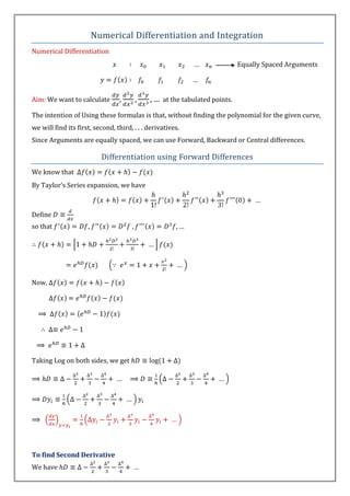
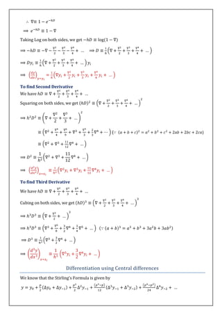
MATHEMATICAL METHODS


NUMERICAL DIFFERENTIATION & INTEGRATION

                            I YEAR B.Tech
                    AS PER JNTU-HYDERABAD NEW SYLLABUS


By
Mr. Y. Prabhaker Reddy
Asst. Professor of Mathematics
Guru Nanak Engineering College
Ibrahimpatnam, Hyderabad.
SYLLABUS OF MATHEMATICAL METHODS (as per JNTU Hyderabad)

Name of the Unit                                      Name of the Topic
                     Matrices and Linear system of equations: Elementary row transformations – Rank
      Unit-I
                     – Echelon form, Normal form       – Solution of Linear Systems    – Direct Methods        – LU
Solution of Linear
                     Decomposition from Gauss Elimination – Solution of Tridiagonal systems – Solution
    systems
                     of Linear Systems.
                     Eigen values, Eigen vectors     – properties   – Condition number of Matrix, Cayley               –
     Unit-II
                     Hamilton Theorem (without proof)       – Inverse and powers of a matrix by Cayley             –
Eigen values and
                     Hamilton theorem       – Diagonalization of matrix Calculation of powers of matrix
                                                                         –                                     –
  Eigen vectors
                     Model and spectral matrices.
                     Real Matrices, Symmetric, skew symmetric, Orthogonal, Linear Transformation -
                     Orthogonal Transformation. Complex Matrices, Hermition and skew Hermition
     Unit-III
                     matrices, Unitary Matrices - Eigen values and Eigen vectors of complex matrices and
     Linear
                     their properties. Quadratic forms - Reduction of quadratic form to canonical form,
Transformations
                     Rank, Positive, negative and semi definite, Index, signature, Sylvester law, Singular
                     value decomposition.
                     Solution of Algebraic and Transcendental Equations- Introduction: The Bisection
                     Method – The Method of False Position       – The Iteration Method - Newton
                                                                                               –Raphson
                     Method Interpolation:Introduction-Errors in Polynomial Interpolation - Finite
     Unit-IV
                     differences- Forward difference, Backward differences, Central differences, Symbolic
Solution of Non-
                     relations and separation of symbols-Difference equations           – Differences of a
 linear Systems
                     polynomial - Newton’s Formulae for interpolation - Central difference interpolation
                     formulae - Gauss Central Difference Formulae - Lagrange’s Interpolation formulae- B.
                     Spline interpolation, Cubic spline.
     Unit-V          Curve Fitting: Fitting a straight line - Second degree curve - Exponential curve -
 Curve fitting &     Power curve by method of least squares.
   Numerical         Numerical Integration: Numerical Differentiation-Simpson’s         3/8    Rule,      Gaussian
   Integration       Integration, Evaluation of Principal value integrals, Generalized Quadrature.
     Unit-VI         Solution   by   Taylor’s s - Picard’s
                                              serie              Method   of   successive     approximation
                                                                                                   - Euler’s
   Numerical         Method -Runge kutta Methods, Predictor Corrector Methods, Adams- Bashforth
 solution of ODE     Method.
                     Determination of Fourier coefficients - Fourier series-even and odd functions -
    Unit-VII
                     Fourier series in an arbitrary interval - Even and odd periodic continuation - Half-
 Fourier Series
                     range Fourier sine and cosine expansions.
    Unit-VIII        Introduction and formation of PDE by elimination of arbitrary constants and
     Partial         arbitrary functions - Solutions of first order linear equation - Non linear equations -
   Differential      Method of separation of variables for second order equations - Two dimensional
   Equations         wave equation.
CONTENTS
UNIT-V
NUMERICAL DIFFERENTIATION & INTEGRATION
          Numerical Differentiation

          Numerical Integration

          Trapezoidal Rule

          Simpson’s 1/3 Rule

            Simpson’s 3/8 Rule
Numerical Differentiation and Integration
Numerical Differentiation
                                                                             Equally Spaced Arguments


Aim: We want to calculate                         at the tabulated points.

The intention of Using these formulas is that, without finding the polynomial for the given curve,
we will find its first, second, third, . . . derivatives.
Since Arguments are equally spaced, we can use Forward, Backward or Central differences.

                           Differentiation using Forward Differences
We know that
By Taylor’s Series expansion, we have


Define
so that              ,


Now,


Taking Log on both sides, we get


To find Second Derivative
We have
Squaring on both sides, we get


                                          (                        )


To find Third Derivative
We have

Cubing on both sides, we get


                      Differentiation using Backward differences
We know that
By Taylor’s Series expansion, we have


Define
so that           ,


Now,
Taking Log on both sides, we get


To find Second Derivative
We have

Squaring on both sides, we get


                                                  (                )


To find Third Derivative

We have

Cubing on both sides, we get


                       Differentiation using Central differences
We know that the Stirling’s Formula is given by
Where

Now, Differentiating w.r.t. , we get


At


Similarly,


When we have to use these formulae?
When we are asked to find         at the point         , the problem analyzing should be as follows:

If the point            is nearer to the starting arguments of the given table, then use Forward
difference formulas for differentiation
If the point            is nearer to the ending arguments of the given table, then use Backward
difference formulas for differentiation
If the point            is nearer to the Middle arguments of the given table, then use Central
difference formulas for differentiation.
Numerical Integration

We know that a definite integral of the form                   represents the area under the curve
             , enclosed between the limits       and         .

Let                  . Here the value of is a Numerical value.
Aim: To find the approximation to the Numerical value of . The process of finding the
approximation to the definite Integral is known as Numerical Integration.
Let                    be given set of observations, and let                  be the corresponding
values for the curve             .


This formulae is also known as Newton Cotes closed type Formulae.
        If        , the formula is known as Trapezoidal Rule
        If        , the formula is known as Simpson’s            Rule
If     , the formula is known as Simpson’s       Rule


Trapezoidal Rule


i.e.

Here   is number of Intervals, and

Simpson’s          Rule


i.e.


Simpson’s         Rule


i.e.
                                       2(                   ℎℎ                   3)

       If Even number of Intervals are there, it is preferred to use Simpson’s    Rule (Or)
       Trapezoidal Rule.
       If Number of Intervals is multiple of 3, then use Simpson’s     Rule (Or) Trapezoidal
       Rule.
       If Odd number of Intervals are there, and which is not multiple of 3, then use Trapezoidal
       Rule. Ex: 5, 7 etc.
       For any number of Intervals, the default Rule we can use is Trapezoidal.

numerical differentiation&integration

  • 1.
    MATHEMATICAL METHODS NUMERICAL DIFFERENTIATION& INTEGRATION I YEAR B.Tech AS PER JNTU-HYDERABAD NEW SYLLABUS By Mr. Y. Prabhaker Reddy Asst. Professor of Mathematics Guru Nanak Engineering College Ibrahimpatnam, Hyderabad.
  • 2.
    SYLLABUS OF MATHEMATICALMETHODS (as per JNTU Hyderabad) Name of the Unit Name of the Topic Matrices and Linear system of equations: Elementary row transformations – Rank Unit-I – Echelon form, Normal form – Solution of Linear Systems – Direct Methods – LU Solution of Linear Decomposition from Gauss Elimination – Solution of Tridiagonal systems – Solution systems of Linear Systems. Eigen values, Eigen vectors – properties – Condition number of Matrix, Cayley – Unit-II Hamilton Theorem (without proof) – Inverse and powers of a matrix by Cayley – Eigen values and Hamilton theorem – Diagonalization of matrix Calculation of powers of matrix – – Eigen vectors Model and spectral matrices. Real Matrices, Symmetric, skew symmetric, Orthogonal, Linear Transformation - Orthogonal Transformation. Complex Matrices, Hermition and skew Hermition Unit-III matrices, Unitary Matrices - Eigen values and Eigen vectors of complex matrices and Linear their properties. Quadratic forms - Reduction of quadratic form to canonical form, Transformations Rank, Positive, negative and semi definite, Index, signature, Sylvester law, Singular value decomposition. Solution of Algebraic and Transcendental Equations- Introduction: The Bisection Method – The Method of False Position – The Iteration Method - Newton –Raphson Method Interpolation:Introduction-Errors in Polynomial Interpolation - Finite Unit-IV differences- Forward difference, Backward differences, Central differences, Symbolic Solution of Non- relations and separation of symbols-Difference equations – Differences of a linear Systems polynomial - Newton’s Formulae for interpolation - Central difference interpolation formulae - Gauss Central Difference Formulae - Lagrange’s Interpolation formulae- B. Spline interpolation, Cubic spline. Unit-V Curve Fitting: Fitting a straight line - Second degree curve - Exponential curve - Curve fitting & Power curve by method of least squares. Numerical Numerical Integration: Numerical Differentiation-Simpson’s 3/8 Rule, Gaussian Integration Integration, Evaluation of Principal value integrals, Generalized Quadrature. Unit-VI Solution by Taylor’s s - Picard’s serie Method of successive approximation - Euler’s Numerical Method -Runge kutta Methods, Predictor Corrector Methods, Adams- Bashforth solution of ODE Method. Determination of Fourier coefficients - Fourier series-even and odd functions - Unit-VII Fourier series in an arbitrary interval - Even and odd periodic continuation - Half- Fourier Series range Fourier sine and cosine expansions. Unit-VIII Introduction and formation of PDE by elimination of arbitrary constants and Partial arbitrary functions - Solutions of first order linear equation - Non linear equations - Differential Method of separation of variables for second order equations - Two dimensional Equations wave equation.
  • 3.
    CONTENTS UNIT-V NUMERICAL DIFFERENTIATION &INTEGRATION  Numerical Differentiation  Numerical Integration  Trapezoidal Rule  Simpson’s 1/3 Rule  Simpson’s 3/8 Rule
  • 4.
    Numerical Differentiation andIntegration Numerical Differentiation Equally Spaced Arguments Aim: We want to calculate at the tabulated points. The intention of Using these formulas is that, without finding the polynomial for the given curve, we will find its first, second, third, . . . derivatives. Since Arguments are equally spaced, we can use Forward, Backward or Central differences. Differentiation using Forward Differences We know that By Taylor’s Series expansion, we have Define so that , Now, Taking Log on both sides, we get To find Second Derivative We have
  • 5.
    Squaring on bothsides, we get ( ) To find Third Derivative We have Cubing on both sides, we get Differentiation using Backward differences We know that By Taylor’s Series expansion, we have Define so that , Now,
  • 6.
    Taking Log onboth sides, we get To find Second Derivative We have Squaring on both sides, we get ( ) To find Third Derivative We have Cubing on both sides, we get Differentiation using Central differences We know that the Stirling’s Formula is given by
  • 7.
    Where Now, Differentiating w.r.t., we get At Similarly, When we have to use these formulae? When we are asked to find at the point , the problem analyzing should be as follows: If the point is nearer to the starting arguments of the given table, then use Forward difference formulas for differentiation If the point is nearer to the ending arguments of the given table, then use Backward difference formulas for differentiation If the point is nearer to the Middle arguments of the given table, then use Central difference formulas for differentiation. Numerical Integration We know that a definite integral of the form represents the area under the curve , enclosed between the limits and . Let . Here the value of is a Numerical value. Aim: To find the approximation to the Numerical value of . The process of finding the approximation to the definite Integral is known as Numerical Integration. Let be given set of observations, and let be the corresponding values for the curve . This formulae is also known as Newton Cotes closed type Formulae. If , the formula is known as Trapezoidal Rule If , the formula is known as Simpson’s Rule
  • 8.
    If , the formula is known as Simpson’s Rule Trapezoidal Rule i.e. Here is number of Intervals, and Simpson’s Rule i.e. Simpson’s Rule i.e. 2( ℎℎ 3) If Even number of Intervals are there, it is preferred to use Simpson’s Rule (Or) Trapezoidal Rule. If Number of Intervals is multiple of 3, then use Simpson’s Rule (Or) Trapezoidal Rule. If Odd number of Intervals are there, and which is not multiple of 3, then use Trapezoidal Rule. Ex: 5, 7 etc. For any number of Intervals, the default Rule we can use is Trapezoidal.