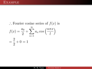
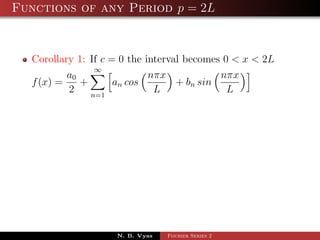
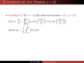
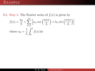
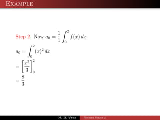
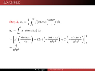
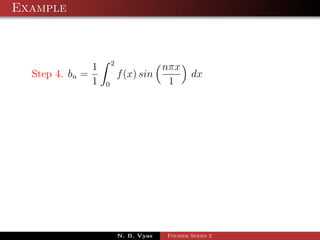
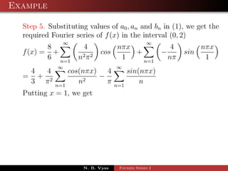
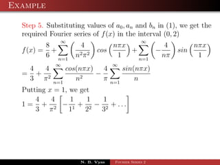
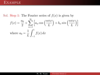
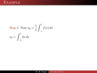
The document discusses the Fourier series representation of periodic functions with an arbitrary period. It provides the general form of the Fourier series for a function f(x) with period 2L, defined over the interval c < x < c + 2L. It also gives the specific forms when c = 0, -L, or L. An example of finding the Fourier series of the function f(x) = x^2 from 0 to 2 is worked out step-by-step.

1. Fourier Series 2
N. B. Vyas
Department of Mathematics,
Atmiya Institute of Tech. & Science,
Rajkot (Guj.)- INDIA
N. B. Vyas Fourier Series 2

2. Functions of any Period p = 2L
Let f (x) be a periodic function with an arbitrary period 2L
defined in the interval c < x < c + 2L
N. B. Vyas Fourier Series 2

3. Functions of any Period p = 2L
Let f (x) be a periodic function with an arbitrary period 2L
defined in the interval c < x < c + 2L
The Fourier series of f (x) is given by
N. B. Vyas Fourier Series 2

4. Functions of any Period p = 2L
Let f (x) be a periodic function with an arbitrary period 2L
defined in the interval c < x < c + 2L
The Fourier series of f (x) is given by
∞
a0 nπx nπx
f (x) = + an cos + bn sin
2 n=1
L L
N. B. Vyas Fourier Series 2

5. Functions of any Period p = 2L
Let f (x) be a periodic function with an arbitrary period 2L
defined in the interval c < x < c + 2L
The Fourier series of f (x) is given by
∞
a0 nπx nπx
f (x) = + an cos + bn sin
2 n=1
L L
c+2L
1
where a0 = f (x) dx
L c
N. B. Vyas Fourier Series 2

6. Functions of any Period p = 2L
Let f (x) be a periodic function with an arbitrary period 2L
defined in the interval c < x < c + 2L
The Fourier series of f (x) is given by
∞
a0 nπx nπx
f (x) = + an cos + bn sin
2 n=1
L L
1 c+2L
where a0 = f (x) dx
L c
1 c+2L nπx
an = f (x) cos dx
L c L
N. B. Vyas Fourier Series 2

7. Functions of any Period p = 2L
Let f (x) be a periodic function with an arbitrary period 2L
defined in the interval c < x < c + 2L
The Fourier series of f (x) is given by
∞
a0 nπx nπx
f (x) = + an cos + bn sin
2 n=1
L L
1 c+2L
where a0 = f (x) dx
L c
1 c+2L nπx
an = f (x) cos dx
L c L
1 c+2L nπx
bn = f (x) sin dx
L c L
N. B. Vyas Fourier Series 2

8. Functions of any Period p = 2L
Corollary 1: If c = 0 the interval becomes 0 < x < 2L
N. B. Vyas Fourier Series 2

9. Functions of any Period p = 2L
Corollary 1: If c = 0 the interval becomes 0 < x < 2L
∞
a0 nπx nπx
f (x) = + an cos + bn sin
2 n=1
L L
N. B. Vyas Fourier Series 2

10. Functions of any Period p = 2L
Corollary 1: If c = 0 the interval becomes 0 < x < 2L
∞
a0 nπx nπx
f (x) = + an cos + bn sin
2 n=1
L L
2L
1
where a0 = f (x) dx
L 0
N. B. Vyas Fourier Series 2

11. Functions of any Period p = 2L
Corollary 1: If c = 0 the interval becomes 0 < x < 2L
∞
a0 nπx nπx
f (x) = + an cos + bn sin
2 n=1
L L
2L
1
where a0 = f (x) dx
L 0
2L
1 nπx
an = f (x) cos dx
L 0 L
N. B. Vyas Fourier Series 2

12. Functions of any Period p = 2L
Corollary 1: If c = 0 the interval becomes 0 < x < 2L
∞
a0 nπx nπx
f (x) = + an cos + bn sin
2 n=1
L L
2L
1
where a0 = f (x) dx
L 0
2L
1 nπx
an = f (x) cos dx
L 0 L
2L
1 nπx
bn = f (x) sin dx
L 0 L
N. B. Vyas Fourier Series 2

13. Functions of any Period p = 2L
Corollary 2: If c = −L the interval becomes −L < x < L
N. B. Vyas Fourier Series 2

14. Functions of any Period p = 2L
Corollary 2: If c = −L the interval becomes −L < x < L
∞
a0 nπx nπx
f (x) = + an cos + bn sin
2 n=1
L L
N. B. Vyas Fourier Series 2

15. Functions of any Period p = 2L
Corollary 2: If c = −L the interval becomes −L < x < L
∞
a0 nπx nπx
f (x) = + an cos + bn sin
2 n=1
L L
L
1
where a0 = f (x) dx
L −L
N. B. Vyas Fourier Series 2

16. Functions of any Period p = 2L
Corollary 2: If c = −L the interval becomes −L < x < L
∞
a0 nπx nπx
f (x) = + an cos + bn sin
2 n=1
L L
1 L
where a0 = f (x) dx
L −L
1 L nπx
an = f (x) cos dx
L −L L
N. B. Vyas Fourier Series 2

17. Functions of any Period p = 2L
Corollary 2: If c = −L the interval becomes −L < x < L
∞
a0 nπx nπx
f (x) = + an cos + bn sin
2 n=1
L L
1 L
where a0 = f (x) dx
L −L
1 L nπx
an = f (x) cos dx
L −L L
1 L nπx
bn = f (x) sin dx
L −L L
N. B. Vyas Fourier Series 2

18. Example
Ex. The Fourier series of f (x) = x2 , 0 < x < 2 where
f (x + 2) = f (x).
N. B. Vyas Fourier Series 2

19. Example
Ex. The Fourier series of f (x) = x2 , 0 < x < 2 where
f (x + 2) = f (x).
1 1 1 π2
Hence deduce that 1 − 2 + 2 − 2 + . . . =
2 3 4 12
N. B. Vyas Fourier Series 2

20. Example
Sol. Step 1: The Fourier series of f (x) is given by
N. B. Vyas Fourier Series 2

21. Example
Sol. Step 1: The Fourier series of f (x) is given by
∞
a0 nπx nπx
f (x) = + an cos + bn sin
2 n=1
L L
N. B. Vyas Fourier Series 2

22. Example
Sol. Step 1: The Fourier series of f (x) is given by
∞
a0 nπx nπx
f (x) = + an cos + bn sin
2 n=1
L L
2
1
where a0 = f (x) dx
L 0
N. B. Vyas Fourier Series 2

23. Example
Sol. Step 1: The Fourier series of f (x) is given by
∞
a0 nπx nπx
f (x) = + an cos + bn sin
2 n=1
L L
1 2
where a0 = f (x) dx
L 0
1 2 nπx
an = f (x) cos dx
L 0 L
N. B. Vyas Fourier Series 2

24. Example
Sol. Step 1: The Fourier series of f (x) is given by
∞
a0 nπx nπx
f (x) = + an cos + bn sin
2 n=1
L L
1 2
where a0 = f (x) dx
L 0
1 2 nπx
an = f (x) cos dx
L 0 L
1 2 nπx
bn = f (x) sin dx
L 0 L
N. B. Vyas Fourier Series 2

25. Example
Sol. Step 1: The Fourier series of f (x) is given by
∞
a0 nπx nπx
f (x) = + an cos + bn sin
2 n=1
L L
1 2
where a0 = f (x) dx
L 0
1 2 nπx
an = f (x) cos dx
L 0 L
1 2 nπx
bn = f (x) sin dx
L 0 L
Here p = 2L = 2 ⇒ L = 1
N. B. Vyas Fourier Series 2

26. Example
2
1
Step 2. Now a0 = f (x) dx
1 0
N. B. Vyas Fourier Series 2

27. Example
2
1
Step 2. Now a0 = f (x) dx
1 0
2
a0 = (x)2 dx
0
N. B. Vyas Fourier Series 2

28. Example
2
1
Step 2. Now a0 = f (x) dx
1 0
2
a0 = (x)2 dx
0
3 2
x
=
3 0
N. B. Vyas Fourier Series 2

29. Example
2
1
Step 2. Now a0 = f (x) dx
1 0
2
a0 = (x)2 dx
0
3 2
x
=
3 0
8
=
3
N. B. Vyas Fourier Series 2

30. Example
2
1 nπx
Step 3. an = f (x) cos dx
1 0 1
N. B. Vyas Fourier Series 2

31. Example
2
1 nπx
Step 3. an = f (x) cos dx
1 0 1
2
an = x2 cos(nπx) dx
0
N. B. Vyas Fourier Series 2

32. Example
2
1 nπx
Step 3. an = f (x) cos dx
1 0 1
2
an = x2 cos(nπx) dx
0
2
sin nπx cos nπx sin nπx
= x2 − (2x) − 2π2
+2 − 3 3
nπ n nπ 0
N. B. Vyas Fourier Series 2

33. Example
2
1 nπx
Step 3. an = f (x) cos dx
1 0 1
2
an = x2 cos(nπx) dx
0
2
sin nπx cos nπx sin nπx
= x2 − (2x) − 2π2
+2 − 3 3
nπ n nπ 0
4
= 2 2
nπ
N. B. Vyas Fourier Series 2

34. Example
2
1 nπx
Step 4. bn = f (x) sin dx
1 0 1
N. B. Vyas Fourier Series 2

35. Example
2
1 nπx
Step 4. bn = f (x) sin dx
1 0 1
2
bn = x2 sin(nπx) dx
0
N. B. Vyas Fourier Series 2

36. Example
2
1 nπx
Step 4. bn = f (x) sin dx
1 0 1
2
bn = x2 sin(nπx) dx
0
2
cos nπx sin nπx cos nπx
= x2 − − (2x) − 2 2 +2
nπ nπ n3 π 3 0
N. B. Vyas Fourier Series 2

37. Example
2
1 nπx
Step 4. bn = f (x) sin dx
1 0 1
2
bn = x2 sin(nπx) dx
0
2
cos nπx sin nπx cos nπx
= x2 − − (2x) − 2 2 +2
nπ nπ n3 π 3 0
4
=−
nπ
N. B. Vyas Fourier Series 2

38. Example
Step 5. Substituting values of a0 , an and bn in (1), we get the
required Fourier series of f (x) in the interval (0, 2)
N. B. Vyas Fourier Series 2

39. Example
Step 5. Substituting values of a0 , an and bn in (1), we get the
required Fourier series of f (x) in the interval (0, 2)
∞ ∞
8 4 nπx 4 nπx
f (x) = + 2π2
cos + − sin
6 n=1 n 1 n=1
nπ 1
N. B. Vyas Fourier Series 2

40. Example
Step 5. Substituting values of a0 , an and bn in (1), we get the
required Fourier series of f (x) in the interval (0, 2)
∞ ∞
8 4 nπx 4 nπx
f (x) = + 2π2
cos + − sin
6 n=1 n 1 n=1
nπ 1
∞ ∞
4 4 cos(nπx) 4 sin(nπx)
= + 2 −
3 π n=1
n2 π n=1
n
N. B. Vyas Fourier Series 2

41. Example
Step 5. Substituting values of a0 , an and bn in (1), we get the
required Fourier series of f (x) in the interval (0, 2)
∞ ∞
8 4 nπx 4 nπx
f (x) = + 2π2
cos + − sin
6 n=1 n 1 n=1
nπ 1
∞ ∞
4 4 cos(nπx) 4 sin(nπx)
= + 2 −
3 π n=1
n2 π n=1
n
Putting x = 1, we get
N. B. Vyas Fourier Series 2

42. Example
Step 5. Substituting values of a0 , an and bn in (1), we get the
required Fourier series of f (x) in the interval (0, 2)
∞ ∞
8 4 nπx 4 nπx
f (x) = + 2π2
cos + − sin
6 n=1 n 1 n=1
nπ 1
∞ ∞
4 4 cos(nπx) 4 sin(nπx)
= + 2 −
3 π n=1
n2 π n=1
n
Putting x = 1, we get
4 4 1 1 1
1 = + 2 − 1 + 2 − 2 + ...
3 π 1 2 3
N. B. Vyas Fourier Series 2

43. Example
Step 5. Substituting values of a0 , an and bn in (1), we get the
required Fourier series of f (x) in the interval (0, 2)
∞ ∞
8 4 nπx 4 nπx
f (x) = + 2π2
cos + − sin
6 n=1 n 1 n=1
nπ 1
∞ ∞
4 4 cos(nπx) 4 sin(nπx)
= + 2 −
3 π n=1
n2 π n=1
n
Putting x = 1, we get
4 4 1 1 1
1 = + 2 − 1 + 2 − 2 + ...
3 π 1 2 3
1 4 1 1 1
− = 2 − 1 + 2 − 2 + ...
3 π 1 2 3
N. B. Vyas Fourier Series 2

44. Example
Step 5. Substituting values of a0 , an and bn in (1), we get the
required Fourier series of f (x) in the interval (0, 2)
∞ ∞
8 4 nπx 4 nπx
f (x) = + 2π2
cos + − sin
6 n=1 n 1 n=1
nπ 1
∞ ∞
4 4 cos(nπx) 4 sin(nπx)
= + 2 −
3 π n=1
n2 π n=1
n
Putting x = 1, we get
4 4 1 1 1
1 = + 2 − 1 + 2 − 2 + ...
3 π 1 2 3
1 4 1 1 1
− = 2 − 1 + 2 − 2 + ...
3 π 1 2 3
2
π 1 1 1 1
= 2 − 2 + 2 − 2 + ...
12 1 2 3 4
N. B. Vyas Fourier Series 2

45. Example
Ex. Find the Fourier series of f (x) = 2x in −1 < x < 1
where p = 2L = 2.
N. B. Vyas Fourier Series 2

46. Example
Sol. Step 1: The Fourier series of f (x) is given by
N. B. Vyas Fourier Series 2

47. Example
Sol. Step 1: The Fourier series of f (x) is given by
∞
a0 nπx nπx
f (x) = + an cos + bn sin
2 n=1
L L
N. B. Vyas Fourier Series 2

48. Example
Sol. Step 1: The Fourier series of f (x) is given by
∞
a0 nπx nπx
f (x) = + an cos + bn sin
2 n=1
L L
1
1
where a0 = f (x) dx
L −1
N. B. Vyas Fourier Series 2

49. Example
Sol. Step 1: The Fourier series of f (x) is given by
∞
a0 nπx nπx
f (x) = + an cos + bn sin
2 n=1
L L
1
1
where a0 = f (x) dx
L −1
1
1 nπx
an = f (x) cos dx
L −1 L
N. B. Vyas Fourier Series 2

50. Example
Sol. Step 1: The Fourier series of f (x) is given by
∞
a0 nπx nπx
f (x) = + an cos + bn sin
2 n=1
L L
1
1
where a0 = f (x) dx
L −1
1
1 nπx
an = f (x) cos dx
L −1 L
1
1 nπx
bn = f (x) sin dx
L −1 L
N. B. Vyas Fourier Series 2

51. Example
Sol. Step 1: The Fourier series of f (x) is given by
∞
a0 nπx nπx
f (x) = + an cos + bn sin
2 n=1
L L
1
1
where a0 = f (x) dx
L −1
1
1 nπx
an = f (x) cos dx
L −1 L
1
1 nπx
bn = f (x) sin dx
L −1 L
Here p = 2L = 2 ⇒ L = 1
N. B. Vyas Fourier Series 2

52. Example
1
1
Step 2. Now a0 = f (x) dx
1 −1
N. B. Vyas Fourier Series 2

53. Example
1
1
Step 2. Now a0 = f (x) dx
1 −1
1
a0 = 2x dx
−1
N. B. Vyas Fourier Series 2

54. Example
1
1
Step 2. Now a0 = f (x) dx
1 −1
1
a0 = 2x dx
−1
=0
N. B. Vyas Fourier Series 2

55. Example
1
1 nπx
Step 3. an = f (x) cos dx
1 −1 1
N. B. Vyas Fourier Series 2

56. Example
1
1 nπx
Step 3. an = f (x) cos dx
1 −1 1
1
an = 2x cos(nπx) dx
−1
N. B. Vyas Fourier Series 2

57. Example
1
1 nπx
Step 3. an = f (x) cos dx
1 −1 1
1
an = 2x cos(nπx) dx
−1
1
sin nπx cos nπx
= 2x − (2) − 2 2
nπ nπ −1
N. B. Vyas Fourier Series 2

58. Example
1
1 nπx
Step 3. an = f (x) cos dx
1 −1 1
1
an = 2x cos(nπx) dx
−1
1
sin nπx cos nπx
= 2x − (2) − 2 2
nπ nπ −1
2(−1)n
= 0+ 2 2
nπ
N. B. Vyas Fourier Series 2

59. Example
1
1 nπx
Step 3. an = f (x) cos dx
1 −1 1
1
an = 2x cos(nπx) dx
−1
1
sin nπx cos nπx
= 2x − (2) − 2 2
nπ nπ −1
n n
2(−1) 2(−1)
= 0+ 2 2 −0− 2 2
nπ nπ
N. B. Vyas Fourier Series 2

60. Example
1
1 nπx
Step 3. an = f (x) cos dx
1 −1 1
1
an = 2x cos(nπx) dx
−1
1
sin nπx cos nπx
= 2x − (2) − 2 2
nπ nπ −1
n n
2(−1) 2(−1)
= 0+ 2 2 −0− 2 2
nπ nπ
=0
N. B. Vyas Fourier Series 2

61. Example
Ex. Find the Fourier series of periodic function
f (x)= −1; −1 < x < 0
= 1; 0 < x < 1
p = 2L = 2
N. B. Vyas Fourier Series 2

62. Example
Ex. Find the Fourier series of periodic function
f (x)= 0; −2 < x < 0
= 2; 0 < x < 2
p = 2L = 4
N. B. Vyas Fourier Series 2

63. Fourier Half Range Series
A function f (x) defined only on the interval of the form
0 < x < L.
N. B. Vyas Fourier Series 2

64. Fourier Half Range Series
A function f (x) defined only on the interval of the form
0 < x < L.
If f (x) is represented on this interval by a Fourier series of
period 2L
N. B. Vyas Fourier Series 2

65. Fourier Half Range Series
A function f (x) defined only on the interval of the form
0 < x < L.
If f (x) is represented on this interval by a Fourier series of
period 2L
Then such Fourier series are known as half range Fourier
series or half range expansions.
N. B. Vyas Fourier Series 2

66. Fourier Half Range Series
A function f (x) defined only on the interval of the form
0 < x < L.
If f (x) is represented on this interval by a Fourier series of
period 2L
Then such Fourier series are known as half range Fourier
series or half range expansions.
Types of Half Range Fourier series
N. B. Vyas Fourier Series 2

67. Fourier Half Range Series
A function f (x) defined only on the interval of the form
0 < x < L.
If f (x) is represented on this interval by a Fourier series of
period 2L
Then such Fourier series are known as half range Fourier
series or half range expansions.
Types of Half Range Fourier series
1 Fourier Cosine Series
N. B. Vyas Fourier Series 2

68. Fourier Half Range Series
A function f (x) defined only on the interval of the form
0 < x < L.
If f (x) is represented on this interval by a Fourier series of
period 2L
Then such Fourier series are known as half range Fourier
series or half range expansions.
Types of Half Range Fourier series
1 Fourier Cosine Series
2 Fourier Sine Series
N. B. Vyas Fourier Series 2

69. Fourier Cosine Series
Let f (x) be piecewise continuous on [o, l].
N. B. Vyas Fourier Series 2

70. Fourier Cosine Series
Let f (x) be piecewise continuous on [o, l].
the Fourier cosine series expansion of f (x) on the half range
interval [0, l] is given by
N. B. Vyas Fourier Series 2

71. Fourier Cosine Series
Let f (x) be piecewise continuous on [o, l].
the Fourier cosine series expansion of f (x) on the half range
interval [0, l] is given by
∞
ao nπx
f (x) = + an cos
2 n=1
l
N. B. Vyas Fourier Series 2

72. Fourier Cosine Series
Let f (x) be piecewise continuous on [o, l].
the Fourier cosine series expansion of f (x) on the half range
interval [0, l] is given by
∞
ao nπx
f (x) = + an cos
2 n=1
l
l
2
where a0 = f (x) dx
l 0
N. B. Vyas Fourier Series 2

73. Fourier Cosine Series
Let f (x) be piecewise continuous on [o, l].
the Fourier cosine series expansion of f (x) on the half range
interval [0, l] is given by
∞
ao nπx
f (x) = + an cos
2 n=1
l
l
2
where a0 = f (x) dx
l 0
l
2 nπx
an = f (x) cos dx
l 0 l
N. B. Vyas Fourier Series 2

74. Fourier Sine Series
Let f (x) be piecewise continuous on [o, l].
N. B. Vyas Fourier Series 2

75. Fourier Sine Series
Let f (x) be piecewise continuous on [o, l].
the Fourier sine series expansion of f (x) on the half range
interval [0, l] is given by
N. B. Vyas Fourier Series 2

76. Fourier Sine Series
Let f (x) be piecewise continuous on [o, l].
the Fourier sine series expansion of f (x) on the half range
interval [0, l] is given by
∞
nπx
f (x) = bn sin
n=1
l
N. B. Vyas Fourier Series 2

77. Fourier Sine Series
Let f (x) be piecewise continuous on [o, l].
the Fourier sine series expansion of f (x) on the half range
interval [0, l] is given by
∞
nπx
f (x) = bn sin
n=1
l
l
2 nπx
bn = f (x) sin dx
l 0 l
N. B. Vyas Fourier Series 2

78. Example
Ex. Find Fourier cosine and sine series of the function
f (x) = 1 for 0 ≤ x ≤ 2
N. B. Vyas Fourier Series 2

79. Example
Sol. Here given interval is 0 ≤ x ≤ 2
N. B. Vyas Fourier Series 2

80. Example
Sol. Here given interval is 0 ≤ x ≤ 2
∴l=2
N. B. Vyas Fourier Series 2

81. Example
1 Fourier cosine series
∞
a0 nπx
Step 1. f (x) = + an cos
2 n=1
l
N. B. Vyas Fourier Series 2

82. Example
1 Fourier cosine series
∞
a0 nπx
Step 1. f (x) = + an cos
2 n=1
l
l
2
where a0 = f (x)dx
l 0
N. B. Vyas Fourier Series 2

83. Example
1 Fourier cosine series
∞
a0 nπx
Step 1. f (x) = + an cos
2 n=1
l
2 l
where a0 = f (x)dx
l 0
2 l nπx
an = f (x) cos
l 0 l
N. B. Vyas Fourier Series 2

84. Example
2
2
Step 2. a0 = f (x)dx
2 0
N. B. Vyas Fourier Series 2

85. Example
2
2
Step 2. a0 = f (x)dx
2 0
2
= 1dx
0
N. B. Vyas Fourier Series 2

86. Example
2
2
Step 2. a0 = f (x)dx
2 0
2
= 1dx = [x]2
0
0
N. B. Vyas Fourier Series 2

87. Example
2
2
Step 2. a0 = f (x)dx
2 0
2
= 1dx = [x]2 = 2.
0
0
N. B. Vyas Fourier Series 2

88. Example
2
2 nπx
Step 3. an = f (x)cos dx
2 0 2
N. B. Vyas Fourier Series 2

89. Example
2 2 nπx
Step 3. an = f (x)cos dx
2 0 2
2
nπx
= (1) cos dx
0 2
N. B. Vyas Fourier Series 2

90. Example
2 2 nπx
Step 3. an = f (x)cos dx
2 0 2
2
nπx
= (1) cos dx
0 2
nπx 2
 
sin
=
 2 
nπ 
2 0
N. B. Vyas Fourier Series 2

91. Example
2 2 nπx
Step 3. an = f (x)cos dx
2 0 2
2
nπx
= (1) cos dx
0 2
nπx 2
 
sin
=
 2 
nπ 
2 0
2
= (sin (nπ) − sin (0))
nπ
N. B. Vyas Fourier Series 2

92. Example
2 2 nπx
Step 3. an = f (x)cos dx
2 0 2
2
nπx
= (1) cos dx
0 2
nπx 2
 
sin
=
 2 
nπ 
2 0
2
= (sin (nπ) − sin (0)) = 0
nπ
N. B. Vyas Fourier Series 2

93. Example
∴ Fourier cosine series of f (x) is
N. B. Vyas Fourier Series 2

94. Example
∴ Fourier cosine series of f (x) is
∞
a0 nπx
f (x) = + an cos
2 n=1
l
N. B. Vyas Fourier Series 2

95. Example
∴ Fourier cosine series of f (x) is
∞
a0 nπx
f (x) = + an cos
2 n=1
l
2
= +0
2
N. B. Vyas Fourier Series 2

96. Example
∴ Fourier cosine series of f (x) is
∞
a0 nπx
f (x) = + an cos
2 n=1
l
2
= +0 =1
2
N. B. Vyas Fourier Series 2