Downloaded 361 times
![DESCRIPTION
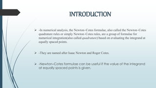
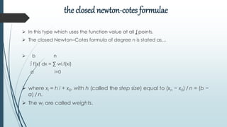
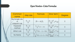
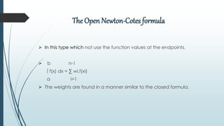
It is assumed that the value of a function ƒ defined on [a, b] is known at
equally spaced points xi, for i = 0, …, n, where x0 = a and xn = b.
Solved Using Newton-Cotes Formulae
There are two types of Newton–Cotes formulae,
1)The "closed" type.
2)The "open" type.](https://image.slidesharecdn.com/newtoncotesitegressionmethod-150620064731-lva1-app6892/85/Newton-cotes-integration-method-3-320.jpg)
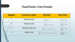
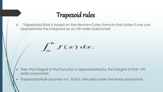
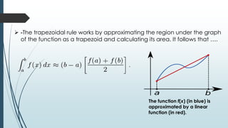
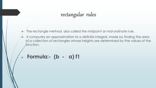
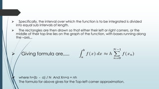
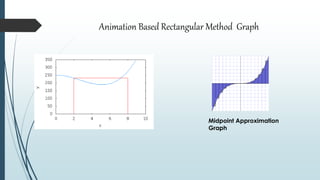
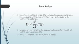


The document discusses the Newton-Cotes integration method, which provides numerical integration formulas using equally spaced points for the evaluation of integrands. It details closed and open types of Newton-Cotes formulas, including specific rules like the trapezoidal rule and Simpson's rule, alongside their applications and error analyses. The document also presents examples to illustrate the application of these methods in practical scenarios.