Numerical integration approximates definite integrals using weighted sums of function values at discretized points. Common integration rules include the rectangular rule, which uses rectangles of width Δx; the trapezoidal rule, which uses trapezoids; and Simpson's rule, which uses a quadratic polynomial to achieve higher accuracy. The document provides examples applying these rules to calculate the integral of f(x)=x^3 from 1 to 2, demonstrating that Simpson's rule provides a perfect estimation while the other rules have some error.

1. Numerical Integration
• In general, a numerical integration is the approximation
of a definite integration by a “weighted” sum of function
values at discretized points within the interval of
integration.
∫
b
a
N
f ( x )dx ≈ ∑ wi f ( xi )
i =0
where wi is the weighted factor depending on the integration
schemes used, and f ( xi ) is the function value evaluated at the
given point xi

2. Rectangular Rule
f(x)
height=f(x1*)
x=a
x=x1*
∫
b
a
height=f(xn*)
x=b
x
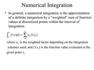
Approximate the integration,
b
∫a f ( x)dx , that is the area under
the curve by a series of
rectangles as shown.
The base of each of these
rectangles is ∆x=(b-a)/n and
its height can be expressed as
f(xi*) where xi* is the midpoint
of each rectangle
x=xn*
f ( x )dx = f ( x1*) ∆x + f ( x2 *) ∆x + .. f ( xn *) ∆x
= ∆x[ f ( x1*) + f ( x2 *) + .. f ( xn *)]

3. Trapezoidal Rule
f(x)
x=a
x=x1
x=b
x=xn-1
x
The rectangular rule can be made
more accurate by using
trapezoids to replace the
rectangles as shown. A linear
approximation of the function
locally sometimes work much
better than using the averaged
value like the rectangular rule
does.
∆x
∆x
∆x
∫a f ( x )dx = 2 [ f (a ) + f ( x1 )] + 2 [ f ( x1 ) + f ( x2 )] + .. + 2 [ f ( xn−1) + f (b)]
1
1
= ∆x[ f (a ) + f ( x1 ) + .. f ( xn −1 ) + f (b)]
2
2
b

4. Simpson’s Rule
Still, the more accurate integration formula can be achieved by
approximating the local curve by a higher order function, such as
a quadratic polynomial. This leads to the Simpson’s rule and the
formula is given as:
∆x
∫a f ( x )dx = 3 [ f (a ) + 4 f ( x1 ) + 2 f ( x2 ) + 4 f ( x3 ) + ..
..2 f ( x2 m−2 ) + 4 f ( x2 m −1 ) + f ( b)]
b
It is to be noted that the total number of subdivisions has to be an
even number in order for the Simpson’s formula to work
properly.

5. Examples
Integrate f ( x ) = x 3 between x = 1 and x = 2.
∫
2
1
1
1
2
x 3dx= x 4 |1 = (24 − 14 ) = 3.75
4
4
2-1
Using 4 subdivisions for the numerical integration: ∆x=
= 0.25
4
Rectangular rule:
i
xi*
f(xi*)
1
1.125 1.42
2
1.375 2.60
3
1.625 4.29
4
1.875 6.59
∫
2
1
x 3dx
= ∆x[ f (1.125) + f (1.375) + f (1.625) + f (1.875)]
= 0.25(14.9) = 3.725

6. Trapezoidal Rule
i
xi
1
f(xi)
1
1 1.25
1.95
2 1.5
3.38
3 1.75
∫
2
1
x 3dx
1
1
f (1) + f (1.25) + f (1.5) + f (1.75) + f (2)]
2
2
= 0.25(15.19) = 3.80
= ∆x[
5.36
2
8
Simpson’s Rule
∫
2
1
x 3dx =
∆x
[ f (1) + 4 f (1.25) + 2 f (1.5) + 4 f (1.75) + f (2)]
3
0.25
=
(45) = 3.75 ⇒ perfect estimation
3

7. Trapezoidal Rule
i
xi
1
f(xi)
1
1 1.25
1.95
2 1.5
3.38
3 1.75
∫
2
1
x 3dx
1
1
f (1) + f (1.25) + f (1.5) + f (1.75) + f (2)]
2
2
= 0.25(15.19) = 3.80
= ∆x[
5.36
2
8
Simpson’s Rule
∫
2
1
x 3dx =
∆x
[ f (1) + 4 f (1.25) + 2 f (1.5) + 4 f (1.75) + f (2)]
3
0.25
=
(45) = 3.75 ⇒ perfect estimation
3