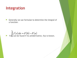
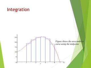
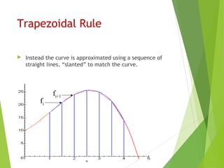
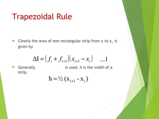
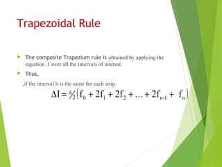
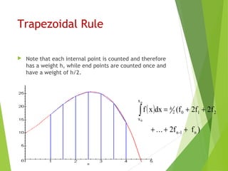
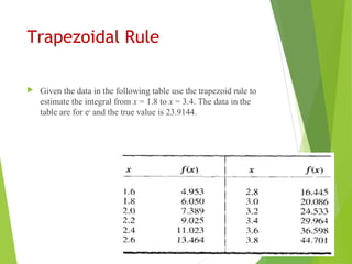
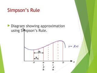
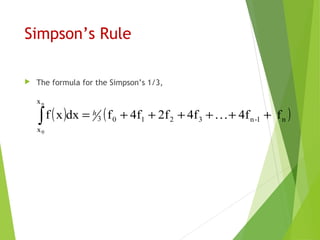
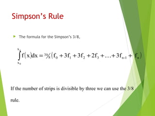
Integration is used in physics to determine rates of change and distances given velocities. Numerical integration is required when the antiderivative is unknown. It involves approximating the definite integral of a function as the area under its curve between bounds. The Trapezoidal Rule approximates this area using straight lines between points, while Simpson's Rule uses quadratic or cubic functions, achieving greater accuracy with fewer points. Both methods involve dividing the area into strips and summing their widths multiplied by the function values at strip points.

1. Numerical
Integration

2. Integration is an important in Physics.
Used to determine the rate of growth in bacteria or to find the
distance given the velocity (s = ∫vdt) as well as many other
uses.
Integration

3. Integration
 Generally we use formulae to determine the integral of
a function:
 F(x) can be found if its antiderivative, f(x) is known.
( ) ( ) ( )aFbFdxxf
b
a
−=∫

4. Integration
 when the antiderivative is unknown we are required to
determine f(x) numerically.
 To determine the definite integral we find the area
between the curve and the x-axis.
 This is the principle of numerical integration.

5. Integration
Figure shows the area under a
curve using the midpoints

6. Integration
 There are various integration methods: Trapezoid,
Simpson’s, etc.
 We’ll be looking in detail at the Trapezoid and variants
of the Simpson’s method.

7. Trapezoidal Rule

8. Trapezoidal Rule
 is an improvement on the midpoint implementation.
 the midpoints is inaccurate in that there are pieces of
the “boxes” above and below the curve (over and under
estimates).

9. Trapezoidal Rule
 Instead the curve is approximated using a sequence of
straight lines, “slanted” to match the curve.
fi
fi+1

10. Trapezoidal Rule
 Clearly the area of one rectangular strip from xi
to xi+1
is
given by
 Generally is used. h is the width of a
strip.
( )( )iiii xxff −+=∆ ++ 11I
)x-(x½h i1i+=
1...

11. Trapezoidal Rule
 The composite Trapezium rule is obtained by applying the
equation .1 over all the intervals of interest.
 Thus,
,if the interval h is the same for each strip.
( )n1-n2102 f2f2f2ffI ++…+++=∆ h

12. Trapezoidal Rule
 Note that each internal point is counted and therefore
has a weight h, while end points are counted once and
have a weight of h/2.
( )
)f2f
2f2f(fdxxf
n1-n
2102
x
x
n
0
++…+
++=∫ h

13. Trapezoidal Rule
 Given the data in the following table use the trapezoid rule to
estimate the integral from x = 1.8 to x = 3.4. The data in the
table are for ex
and the true value is 23.9144.

14. Trapezoidal Rule
 As an exercise show that the approximation given by the
trapezium rule gives 23.9944.

15. Simpson’s Rule

16. Simpson’s Rule
 The midpoint rule was first improved upon by the
trapezium rule.
 A further improvement is the Simpson's rule.
 Instead of approximating the curve by a straight line,
we approximate it by a quadratic or cubic function.

17. Simpson’s Rule
 Diagram showing approximation
using Simpson’s Rule.

18. Simpson’s Rule
 There are two variations of the rule: Simpson’s 1/3 rule
and Simpson’s 3/8 rule.

19. Simpson’s Rule
 The formula for the Simpson’s 1/3,
( ) ( )n1-n32103
x
x
f4f4f2f4ffdxxf
n
0
++…++++=∫ h

20. Simpson’s Rule
 The integration is over pairs of intervals and requires
that total number of intervals be even of the total
number of points N be odd.

21. Simpson’s Rule
 The formula for the Simpson’s 3/8,
( ) ( )n1-n32108
3
x
x
f3f2f3f3ffdxxf
n
0
++…++++=∫ h
If the number of strips is divisible by three we can use the 3/8
rule.

22. Thank You