Engineering Mathematics-IV_B.Tech_Semester-IV_Unit-V

Numerical Integration
and
Numerical Differentiation
Course- B.Tech
Semester-IV
Subject- ENGINEERING MATHEMATICS-IV
Unit- V
RAI UNIVERSITY, AHMEDABAD

Unit-V Numerical Integration and Numerical Differentiation
Content
NUMERICAL INTEGRATION—Trapezoidal method & it’s problems method, Simpson’s one
third and three-eight rules & Problem based on Simpson’s one third and three-eight rules.
NUMERICAL DIFFERENTIATION—Solution of ordinary differential equations by following
methods: Euler’s Method, Picard’s Method and forth-order Runge- Kutta methods & it’s
problems

1.1 Numerical Integration— The process of evaluating a definite integral from a set of
tabulated values of the integrand ( ) is called numerical integration. When this process is
applied to a function of single function is called quadrature.
Consider the definite integral∫ ( ) representsthe area between = ( ) with random
= and = .This integration is possible only when ( ) is explicitly given or otherwise it
is not possible to evaluate.
In numerical integration for given set of ( + 1) paired values of the function taking the
values , , … corresponding to the values , , … , where ( ) is not known
explicitly, it is possible to compute∫ ( ) by numerical integration by using various method.
1. Trapezoidal method
2. Simpson’s one third rule
3. Simpson’s three-eight rule
1.2 Newton-Cote’s quadrature— Let
= ( )
Where ( ) takes the values , , … , for , , … divide the interval ( , ) into n
sub-interval of width h, so that = , = + ℎ, = + 2ℎ, = + ℎ = .
Then = ∫ ( )
Putting = + ℎ
⟹ = ℎ
∴ = ℎ ( + ℎ)
By Newton’s forward interpolation formula
= ℎ + ∆ +
( − 1)
2!
∆ +
( − 1)( − 3)
3!
∆ + ⋯
Integration term by term, we get

( )
= ℎ +
2
∆ +
(2 − 3)
12
∆ +
( − 2)
24
∆ + ⋯ … … ( )
This equation is known as Newton-Cote’s quadrature formula. Being a general formula, we
deduce many formula’s from this by taking = 1,2,3 …
1.3 Trapezoidal method— Assume that ( ) is continuous on [ , ] and divide [ , ] into n
subinterval of equal length.
∆ =
−
Using ( + 1) points = , = + ∆ , = + 2∆ , = + ∆ =
Computing the values of ( ) at these points
= ( ), = ( ), = ( ), = ( )
Approximate integral by using n trapezoids formed by using straight line segments between two
points ( , ) and ( , ) for 1 ≤ ≤ as shown in the figure:
Area of a trapezoid is obtained by adding the areas of rectangles and triangles.
= ∆ +
1
2
( − )∆ =
( )∆
2
Adding area of the n trapezoids, the approximation is
( ) ≈
( + )∆
2
+
( + )∆
2
+
( + )∆
2
+ ⋯ +
( + )∆
2

This simplifies the trapezoidal rule.
( ) ≈
∆
2
( + 2 + 2 + ⋯ + 2 + )
≈
∆
[( + ) + 2( + + ⋯ + )]
We can also replace ∆ withℎ. So the formula will be
( ) =
ℎ
2
[( + ) + 2( + + ⋯ + )]
≈ [( ℎ ) + 2( ℎ )]
Another Procedure—
Putting = 1in ( ) and taking the curve through ( , ) and ( , ) as straight line. i.e.
Polynomial of first order so that differences of order higher than first become zero, we get
( ) = ℎ +
1
2
∆ =
ℎ
2
( + )
Similarly
( ) = ℎ +
1
2
∆ =
ℎ
2
( + )
⋮
( ) =
ℎ
2
( )
( + )
Adding these n integrals, we obtain
( ) =
ℎ
2
[( + ) + 2( + + ⋯ + )]
This is known as the trapezoidal rule.

Example—Evaluate∫ by using Trapezoidal rule. Verify result by actual integration.
Solution—given that ( ) =
Interval length ( – ) = (3 – (−3) ) = 6
So we divide 6 equal intervals with ℎ = 6/6 = 1.0
And tabulate the values as below
-3 -2 -1 0 1 2 3
= 81 16 1 0 1 16 81
We know that—
( ) ≈
ℎ
2
[( + ) + 2( + + ⋯ + )]
≈
1
2
[(81 + 81) + 2 (16 + 1 + 0 + 1 + 16)] =
162 + 68
2
= 115
By actual integration ∫ = − − = + = = 97.5
Example— Evaluate ∫ ( )
by using Trapezoidal rule with h = 0.2.
Solution— Given ( ) = ( )
and interval length ( – ) = (1 – 0 ) = 1.
So we divide 6 equal intervals with h= 0.2
We know ∫ ( ) ≈ [( + ) + 2( + + ⋯ + )]
1
(1 + )
≈
0.2
2
[(1 + 0.5000) + 2(0.96154 + 0.86207 + 0.73529 + 0.60976)]
=(0.1)[ (1.05) + 6.33732 ]
= 0.783732
0 0.2 0.4 0.6 0.8 1
y =
1
(1 + x )
1 0.96154 0.86207 0.73529 0.60976 0.5000

1.4 Simpson’s one third rule— Putting = 2 in ( ) and taking the curve through
( , ), ( , ) and ( , ) as a parabola, i.e. a polynomial of second order so that differences
of higher than second vanish, we get
( ) = 2ℎ + ∆ +
1
6
∆ =
ℎ
3
( + 4 + )
Similarly
( ) =
ℎ
3
( + 4 + )
⋮
∫ ( ) =( )
( + 4 + ), is even.
Adding these n integrals, we have when is even
( ) =
ℎ
3
[( + ) + 4( + + ⋯ + ) + 2( + + ⋯ + )]
=(ℎ/3) [ (sum of the irst and last ordinates ) + 2 (Sum of remaining even ordinates)
+4 ( sum of remaining odd ordinates) ]
This is known as the Simpson’s one third rule or simply Simpson’s rule.
1.4 Simpson’s three-eight rule — Putting = 3 in ( ) and taking the curve through
( , ): = 0,1,2,3 as polynomial of third order so that the differences above the third order
vanish, we get
( ) = 3ℎ +
3
2
∆ +
3
2
∆ +
1
8
∆ =
3ℎ
8
( + 3 + 3 + )
Similarly, ∫ ( ) = ( + 3 + 3 + ) and so on.
adding all these expressions from to + ℎ, where n is multiple of 3, we obtain
( ) =
3ℎ
8
[( + ) + 3( + + + … + ) + 2( + + ⋯ + )]
= (3ℎ/8) [ (sum of the irst and last ordinates )
+ 2 (Sum of multiples of three ordinates) + 3 ( sum of remaining ordinates)]
Which is known as Simpson’s three-eight rule.

Example— Evaluate∫ by using Simpson’s one third rule and Simpson’s three-eight
rule. Verify result by actual integration.
Solution—We are given that ( ) =
Interval length ( – ) = (3 – (−3) ) = 6
So we divide 6 equal intervals with ℎ = 6/6 = 1.0 and tabulate the values as below
-3 -2 -1 0 1 2 3
= 81 16 1 0 1 16 81
By Simpson’s one third rule
=
ℎ
3
[( + ) + 4( + + ) + 2( + )]
= [(81 + 81) + 4(16 + 0 + 16) + 2(1 + 1)] = = 98
By Simpson’s three-eight rule
=
3ℎ
8
[( + ) + 3( + + + ) + 2 )]
= [(81 + 81) + 3(16 + 1 + 1 + 16) + 2 × 0] = = 99
By actual integration ∫ x dx = − − = + = = 97.5
Example—Evaluate∫
.
by using Trapezoidal rule, Simpson’s one third rule and
Simpson’s three-eighth rule.
Solution—We are given that ( ) = Interval length ( – ) = (5.2 – 4 ) = 1.2.So
we divide 6 equal intervals with ℎ = 0.2 and tabulate the values as below
4.0 4.2 4.4 4.6 4.8 5.0 5.2
= 1.39 1.44 1.48 1.53 1.57 1.61 1.65
By Trapezoidal rule
=
.
ℎ
2
[( + ) + 2( + + ⋯ + )]
=
0.2
2
[(1.39 + 1.65) + 2 (1.44 + 1.48 + 1.53 + 1.57 + 1.61)]
= (0.1) [ 3.04 + 2(7.63) ]
= 1.83

By Simpson’s one third rule
.
=
ℎ
3
[( + ) + 4( + + ) + 2( + )]
= (0.2/3) [ (1.39 + 1.65) + 2 (1.48 + 1.57) + 4 (1.44 + 1.53 + +1.61) ]
= (0.0667) [ 3.04 + 2(3.05) + 4 (4.58) ]
= 1.83
By Simpson’s three-eight rule
.
=
3ℎ
8
[( + ) + 3( + + + ) + 2 )]
= (
× .
)[ (1.39 + 1.65) + 2 (1.53) + 3 (1.44 + 1.48 + 1.57 + +1.61) ]
= (0.075 ) [ 3.04 + 3.06 + 3 (6.1) ]
= 1.83
2 Numerical Differentiations—
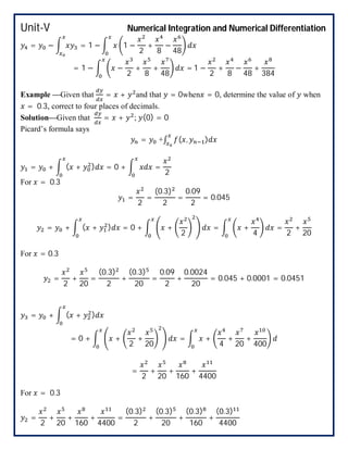
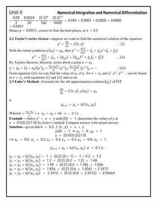
2.1 Picard’s Method— Let us considers the first order differential equation = ( , ) and
( ) = then from the Picard’s method, nth
approximation to the solution of Initial value
problem eq (i) is
= +∫ ( , )
Example —Use Picard’s method to solve = − upto the fourth approximation, when
(0) = 1.
Solution—Given differential equation is = − , when (0) = 1.
Picard’s formula says
= +∫ ( , )
= − = 1 − × 1 = 1 −
2
= − = 1 − 1 −
2
= 1 − −
2
= 1 −
2
+
8
= − = 1 − 1 −
2
+
8
= 1 − −
2
+
8
= 1 −
2
+
8
−
48

= − = 1 − 1 −
2
+
8
−
48
= 1 − −
2
+
8
+
48
= 1 −
2
+
8
−
48
+
384
Example —Given that = + and that = 0when = 0, determine the value of when
= 0.3, correct to four places of decimals.
Solution—Given that = + ; (0) = 0
Picard’s formula says
= +∫ ( , )
= + ( + ) = 0 + =
2
For = 0.3
=
2
=
(0.3)
2
=
0.09
2
= 0.045
= + ( + ) = 0 + +
2
= +
4
=
2
+
20
For = 0.3
=
2
+
20
=
(0.3)
2
+
(0.3)
20
=
0.09
2
+
0.0024
20
= 0.045 + 0.0001 = 0.0451
= + ( + )
= 0 + +
2
+
20
= +
4
+
20
+
400
=
2
+
20
+
160
+
4400
For = 0.3
=
2
+
20
+
160
+
4400
=
(0.3)
2
+
(0.3)
20
+
(0.3)
160
+
(0.3)
4400

=
0.09
2
+
0.0024
20
+
(0.3)
160
+
(0.3)
4400
= 0.045 + 0.0001 + 0.0000 + 0.0000
= 0.0451
Hence, = 0.0451, correct to four decimal places, at = 0.3
2.2 Taylor’s series Method—suppose we want to find the numerical solution of the equation
= = ( , ) … ( )
With the initial condition ( ) = , then = = + = +
= = + 2 + 2 + + … ( )
By Taylors theorem, theorem, series about a point =
= + ( − )( ) +
( )
!
( ) +
( )
!
( ) + ⋯ … ( )
From equation ( ) we can find the value of of for = and , , … can be found
at = with equations ( ) and ( ) and so on.
2.3 Euler’s Method—Formula for the nth approximation solution( ) of IVP
= ( , ), ( ) =
is
= + ℎ ( , )
Whereℎ = . . = + ℎ ; = 0,1,2, …
Example —Solve = + and (0) = 1, determine the values of y at
= 0.0(0.2)(1.0) by Euler’s method. Compare answer with actual answer.
Solution—given that ℎ = 0.2 , ( , ) = +
(0) = 1 ⇒ = 0 , = 1
= (0.0)(0.2)(1.0)
⟹ = 0.0 , = 0.2, = 0.4, = 0.4, = 0.8 , = 1.
= + ℎ ( , ) , = 0,1,2, …
= + ℎ ( , ) = 1 + (0.2) (0 + 1) = 1 + 0.2 = 1.2
= + ℎ ( , ) = 1.2 + (0.2) (0.2 + 1.2) = 1.48
= + ℎ ( , ) = 1.48 + (0.2) (0.4 + 1.48) = 1.856
= + ℎ ( , ) = 1.856 + (0.2) (0.6 + 1.856) = 2.3472
= + ℎ ( , ) = 2.3472 + (0.2) (0.8 + 2.3472) = 2.94664

2.4 Modified Euler’s method— Formula for this method up to nth
approximation to solution of
IVP
= + [ ( , ) + ( , )], = 0,1,2, …
Where is calculated by using Euler’s method.
i.e.
= + ℎ ( , )
Example—Use Modified Euler’s Method to compute for = 2, Given that = + ,
= 0, = 1 with ℎ = 1.
Solution—Formula for Modified Euler’s method is
= + [ ( , ) + ( , )], = 0,1,2, …
Since Euler formula is = + ℎ ( , )
Here we write in place of .
= + ℎ ( , )
= + + = + 2 ∵ ℎ = 1
Value of
= + 2 = 0 + 2 = 2
⟹ = +
1
2
[ ( , ) + ( , )]
= + [ + + + ]
= + [0 + 1 + 1 + 2] = 1 + 2 = 3
(∵ = + ℎ = 0 + 1 = 1)
Value of
= + 2 = 1 + 2 × 3 = 7
⟹ = +
1
2
[ ( , ) + ( , )]
= + [ + + + ]
= 3 + [1 + 3 + 2 + 7] = 3 + =
Example —Solve numerically ’ = + , (0) = 0, for = 0.2, 0.4by modified Euler’s
method.
Solution—We are given that ’ = + , (0) = 0 ; ( , ) = + .
(0) = 0 ⟹ = 0 , = 0
= 0.2, 0.4 ⟹ = 0.0 , = 0.2, = 0.4 and ℎ = 0.2
Formula for Modified Euler’s method is
= + [ ( , ) + ( , )], = 0,1,2, …

Where is calculated by using Euler’s method—
= + ℎ ( , ) = + (0.2)( + )
Value of
= + (0.2)( + ) = 0 + (0.2)(0 + 1) = 0.2
⟹ = + [ ( , ) + ( , )]
= + [ + + + ]
= 0 +
.
[ 0 + + 0.2 + .
]
= 0 + 0.1[ 0 + 1 + 0.2 + 1.2214]
= 0.24214
Value of
= + (0.2)( + ) = 0.24214 + (0.2)(0.24214 + . )
= 0.24214 + (0.2)(0.24214 + 1.2214) = 0.24214 + (0.2)(1.4635)
= 0.24214 + 0.2927 = 0.53485
⟹ = +
ℎ
2
[ ( , ) + ( , )]
= + [ + + + ]
= 0.24214 +
.
[0.24214 + .
+ 0.53485 + . ]
= 0.24214 + 0.1[0.24214 + 1.2214 + 0.53485 + 1.4918]
= 0.24214 + 0.1(3.49019) = 0.24214 + 0.349019 = 0.59116
2.5 Runge-Kutta Method—
1. Euler method is the Runge-Kutta Method of first order.
2. Modified Euler method is the Runge-Kutta Method of second order.
2.5.1 Third order of R-K Method—
= +
1
6
( + 4 + )
Where—
= ℎ 0, 0 ,
= ℎ 0 +
ℎ
2
, 0 + 2
and
= ℎ 0 + ℎ, 0 + ℎ 0 + ℎ, 0 + 1
2.5.2 Fourth order of R-K Method—
This method is most commonly used and is generally called as Runge-Kutta Method only.
In the initial problem
= ( , ), ( ) =
Approximate value of y is given as = + where
=
1
6
( + + + )

and
= ℎ 0, 0
= ℎ 0 +
ℎ
2
, 0 + 1
2
= ℎ 0 +
ℎ
2
, 0 + 2
2
4 = ℎ ( + ℎ, + 3)
Note— ( , ) = ( ), . . , ( , ) is only depending on a function x alone, then the
fourthorder Runge-Kutta method reduces toSimpson’s one third rule.
Example—Apply Runge-Kutta method to find an approximation value of , when = 0 given
that = + , = 0,when = 0 with ℎ = 0.1
Solution— Here = 0, = 1, ( , ) = +
Now
= ℎ 0, 0 = 0.1(0 + 1) = 0.1
= ℎ +
ℎ
2
, +
ℎ
2
= 0.1 (0 + 0.05,1 + 0.05) = 0.1[0.05 + 1.05] = 0.1 × 1.1
= 0.11
= ℎ +
ℎ
2
, +
2
= 0.1 (0 + 0.05,1 + 0.055) = 0.1[0.05 + 1.055] = 0.1 × 1.105
= 0.1105
= ℎ ( + ℎ, + ) = 0.1 (0 + 0.1,1 + 0.1105) = 0.1(0.1 + 1.1105) = 0.1 × 1.2105
= 0.12105
According to Runge-Kutta fourth order formula
=
1
6
( + 2 + 2 + ) =
1
6
[0.1 + 2(0.11) + 2(0.1105) + 0.12105]
=
1
6
(0.1 + 0.22 + 0.221 + 0.12105) =
1
6
(0.66205) = 0.11034
= +
. = 1 + 0.11034 = 1.11034
Example —Obtain the values of y at x= 0.1, 0.2 using R.K. method of fourth order for the
differential equation = − , given y(0) =1.
Solution—we are given that = − , (0) = 1
⟹ ( , ) = − , = 0 , = 1
Since h is clearly specified in the question, we take ℎ = 0.1; = 0.1, = 0.2
= ℎ 0, 0 = 0.1(−1) = −0.1

= h +
ℎ
2
, +
2
= 0.1 0 + 0.05,1 +
−0.1
2
= 0.1 (0.05,0.95) = 0.1(−0.95)
= −0.095
= ℎ 0 +
ℎ
2
, 0 + 2
2
= 0.1 0 + 0.05,1 +
−0.095
2
= 0.1 (0.05,0.9525)
= 0.1(−0.9525) = −0.09525
= ℎ ( + ℎ, + ) = 0.1 0 + 0.1,1 + (−0.09525) = 0.1 (0.1,0.90475)
= − 0.090475
According to Runge-Kutta fourth order formula
k =
1
6
(k + 2k + 2k + k )
= [(−0.095) + 2(−0.095) + 2(−0.09525) + (− 0.090475)]
= [−0.095 − 0.19 − 0.1925 − 0.090475] =
.
= − 0.094329166
y = y + k
y . = 1 + (− 0.094329166) = 0.905670833

Exercise
1. If = 2 − and = 2when = 1, perform three iterations of Picard’s method to estimate a value
for y when x= 1.2. Work to four places of decimals throughout and state how accurate is the result of the
third iteration.
2. Solve ′ = − ,and y(0) = 1, determine the values of y at x =(0.01)(0.01)(0.04) by Euler’s method.
3. Obtain the values of y at x= 0.1, 0.2 using R.K. method of fourth order for the differential equation ′
=
− , given y(0) =1.5.
4. Apply Rungakutta method to find an approximation value of , when = 0 given that = − , =
0,when = 0 with ℎ = 0.1
5. Find y (0.2) given = – , (0) = 2 taking h = 0.1. by Runge –Kutta method.
6. Evaluate y(1.4) given = + , (1.2) = 2. By Runge-Kutta Method.

Reference
1. http://en.wikipedia.org/wiki/File:Integral_as_region_under_curve.svg
2. http://www.google.co.in/url?sa=i&rct=j&q=&esrc=s&source=images&cd=&cad=rja&uact=8&ved=0CAcQ
jRw&url=http%3A%2F%2Fcalculator.mathcaptain.com%2Ftrapezoidal-rule-
calculator.html&ei=z7qnVKa5DsiNuATbtoHoCQ&bvm=bv.82001339,d.c2E&psig=AFQjCNHqSN98kFMHM
wdx482zLm5KtRJA6A&ust=1420364847649006
3. Numerical Method for Science and Computer science by M.K. Jain, S.R.K. Iyenger, R.K. Jain
4. Higher Engineering Mathematics, B.S. Grewal, Khanna Publishers.
5. Higher Engineering Mathematics, B V Ramana, McGraw Hill Education

Engineering Mathematics-IV_B.Tech_Semester-IV_Unit-V

More Related Content

What's hot

Viewers also liked

Similar to Engineering Mathematics-IV_B.Tech_Semester-IV_Unit-V

More from Rai University

Recently uploaded

Engineering Mathematics-IV_B.Tech_Semester-IV_Unit-V