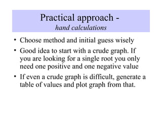
Downloaded 850 times
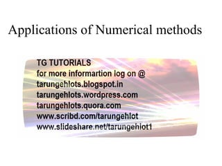


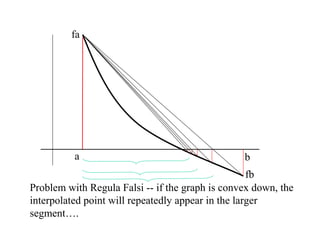


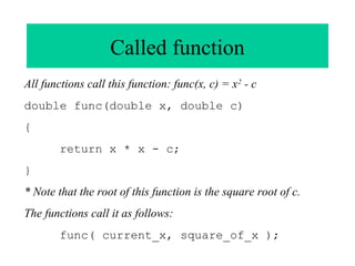
![Modified Regula Falsi
• If the root is in the left segment [a, interior]
– Draw line between (a, fa*0.5) and (interior, finterior)
• Else (in the right segment [interior, b])
-- Draw line between (interior, finterior) and (b, fb*0.5)
fb
a
interior2
interior3
fa
interior1
b](https://image.slidesharecdn.com/applicationsofnumericalmethods-131111131023-phpapp02/85/Applications-of-numerical-methods-29-320.jpg)


![Important differences from text
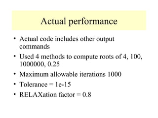
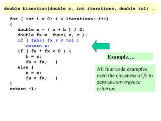
• Assumed all methods would be used to find
square root of k between [1, c] or [c,1] by
finding root of x2 – c.
• All used closeness of fx to 0 as convergence
criteria. Text uses different criteria for
different algorithms](https://image.slidesharecdn.com/applicationsofnumericalmethods-131111131023-phpapp02/85/Applications-of-numerical-methods-43-320.jpg)
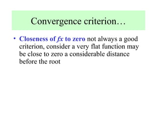
![Other convergence criteria
• Width of the interval [a,b]. If this interval
contains the root, guaranteed that the root is
within this much accuracy
• However, interval does not necessarily
contain the root (secant method)
• Text uses the width of the interval as the
convergence criteria in the Bisection
Method](https://image.slidesharecdn.com/applicationsofnumericalmethods-131111131023-phpapp02/85/Applications-of-numerical-methods-46-320.jpg)
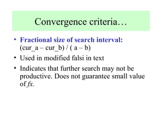
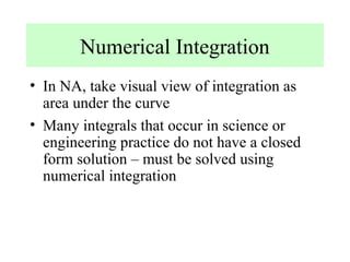
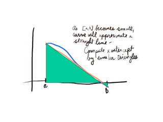
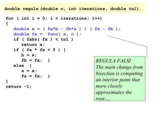
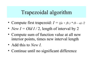
![Trapezoidal Rule
• The area under the curve from
[a, fa] to [b, fb] is initially approximated by
a trapezoid:
I1 = ( b – a ) * ( fa + fb ) / 2](https://image.slidesharecdn.com/applicationsofnumericalmethods-131111131023-phpapp02/85/Applications-of-numerical-methods-49-320.jpg)


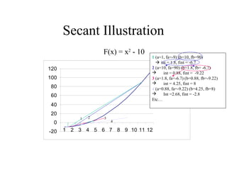
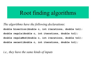
The document discusses numerical methods for finding roots of equations and integrating functions. It covers root-finding algorithms like the bisection method, Regula Falsi method, modified Regula Falsi, and secant method. These algorithms iteratively find roots by narrowing the interval that contains the root. The document also discusses numerical integration techniques like the trapezoidal rule to approximate the area under a curve without having a closed-form solution. It notes the tradeoffs between different root-finding algorithms in terms of speed, accuracy, and ability to guarantee convergence.


