23MA401 NM Unit 3 Numerical integration anddifferenciation

1. 23MA401- Numerical Methods
Numerical Differentiation and
Integration
By
Dr. S.Shyamala AP/Maths
Ms.G. Nandhini AP/Maths
Excel Engineering College (Autonomous)

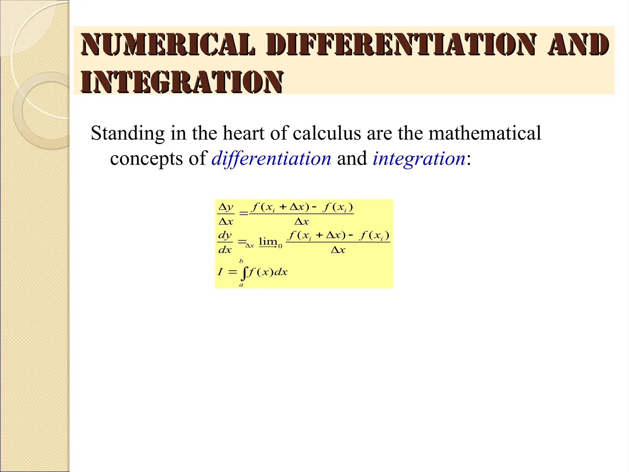
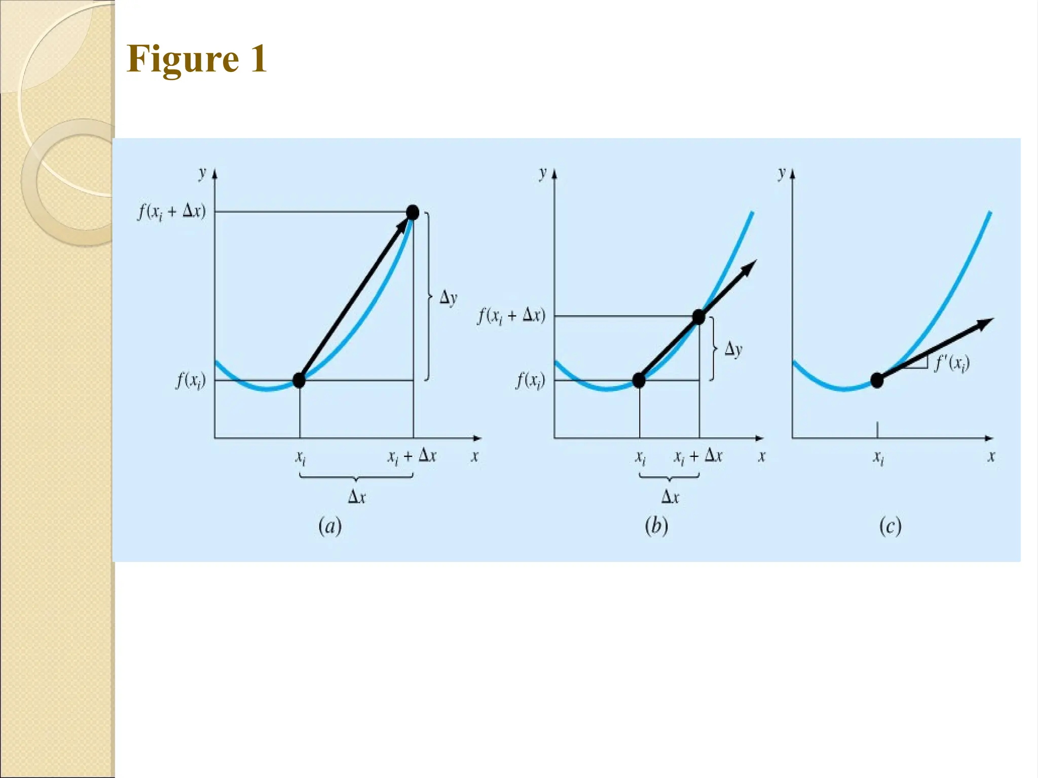
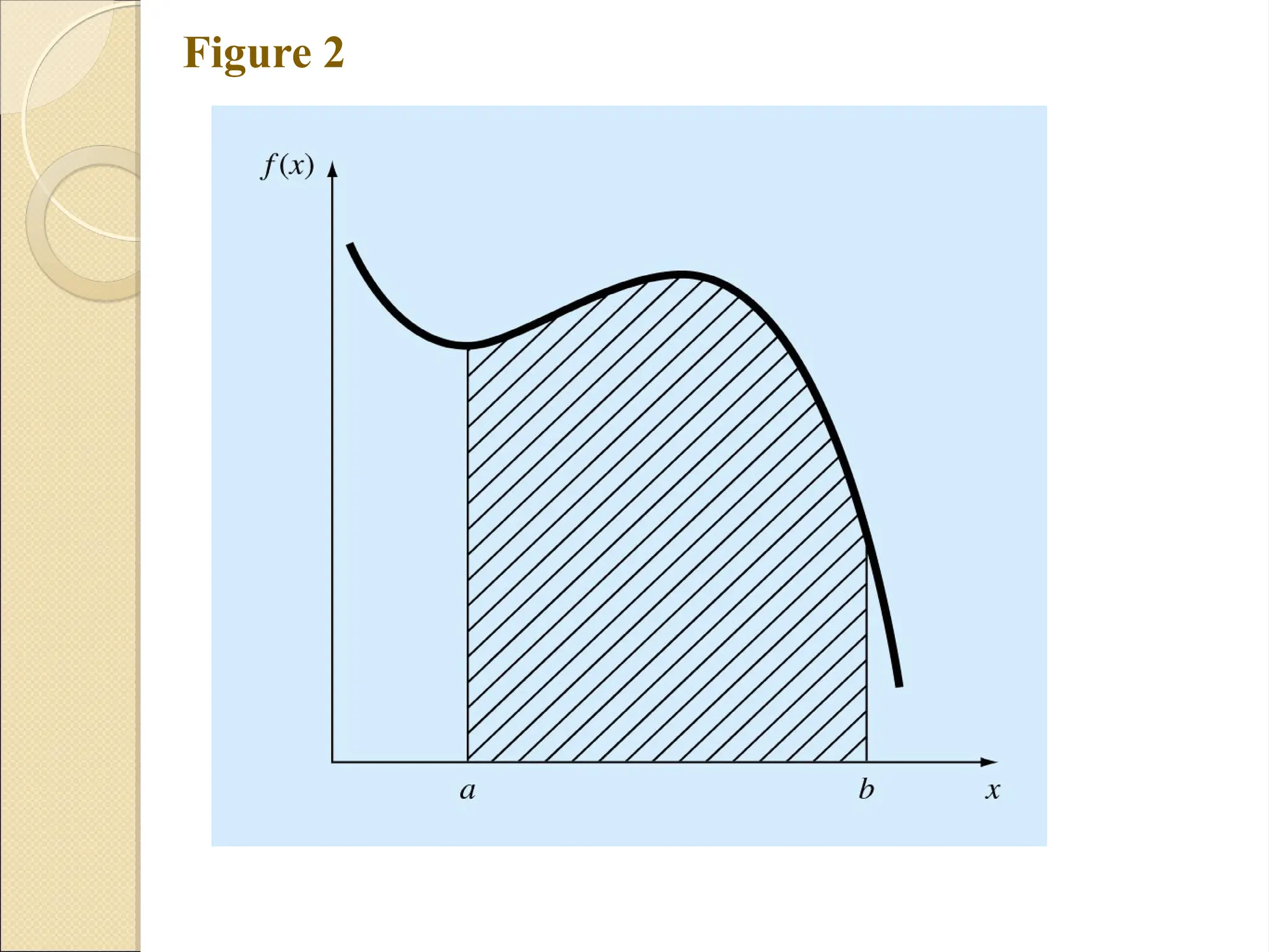
2. Copyright © 2006 The McGraw-Hill Companies, Inc. Permission required for reproduction or display.
Numerical Differentiation and
Numerical Differentiation and
Integration
Integration















b
a
i
i
x
i
i
dx
x
f
I
x
x
f
x
x
f
dx
dy
x
x
f
x
x
f
x
y
)
(
)
(
)
(
lim
)
(
)
(
0
Standing in the heart of calculus are the mathematical
concepts of differentiation and integration:

3. Copyright © 2006 The McGraw-Hill Companies, Inc. Permission required for reproduction or display.
Figure 1

4. Copyright © 2006 The McGraw-Hill Companies, Inc. Permission required for reproduction or display.
Figure 2

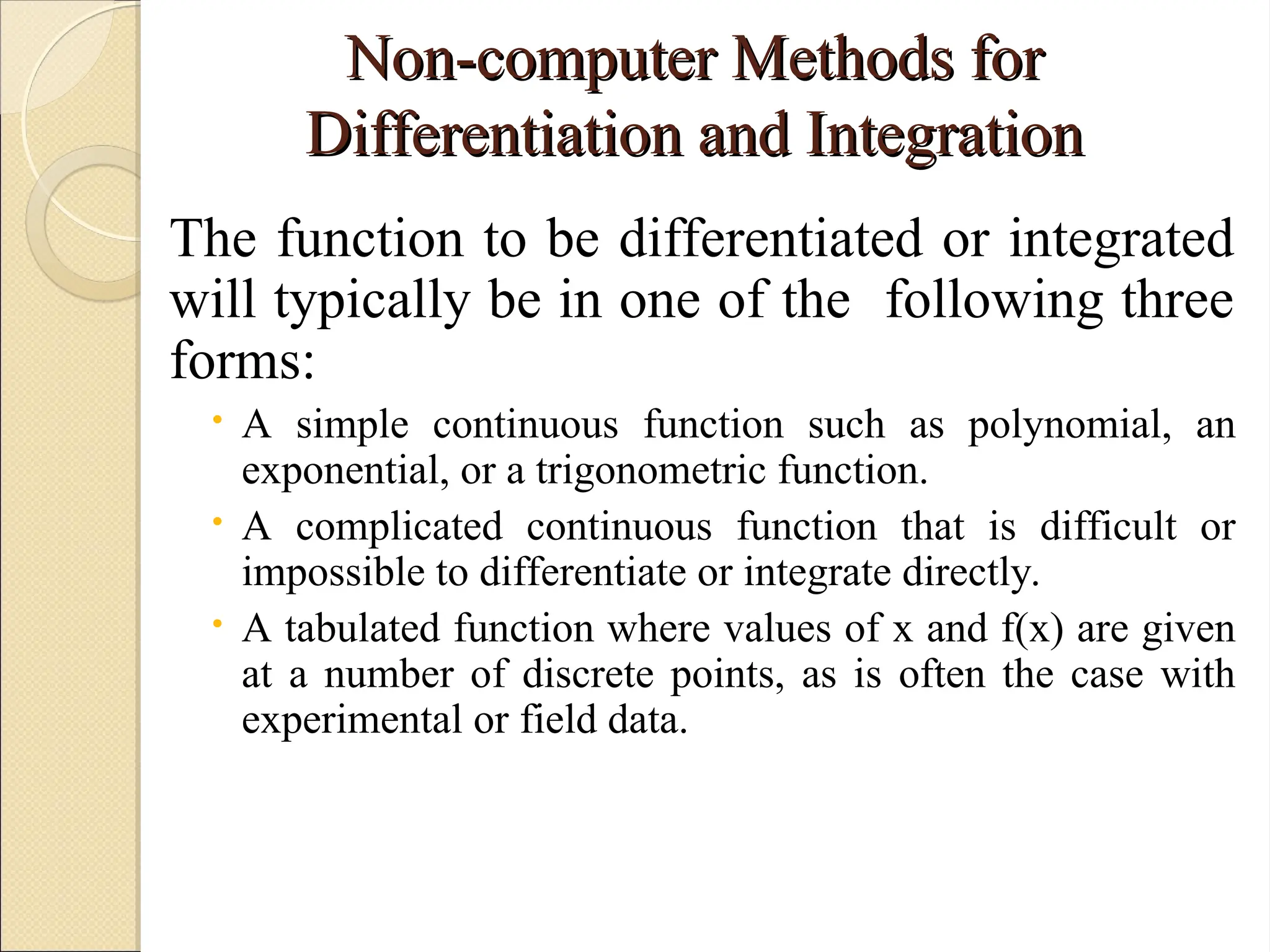
5. Copyright © 2006 The McGraw-Hill Companies, Inc. Permission required for reproduction or display.
Non-computer Methods for
Non-computer Methods for
Differentiation and Integration
Differentiation and Integration
The function to be differentiated or integrated
will typically be in one of the following three
forms:
 A simple continuous function such as polynomial, an
exponential, or a trigonometric function.
 A complicated continuous function that is difficult or
impossible to differentiate or integrate directly.
 A tabulated function where values of x and f(x) are given
at a number of discrete points, as is often the case with
experimental or field data.

6. Copyright © 2006 The McGraw-Hill Companies, Inc. Permission required for reproduction or display.
Figure 3

7. Copyright © 2006 The McGraw-Hill Companies, Inc. Permission required for reproduction or display.
Figure 4

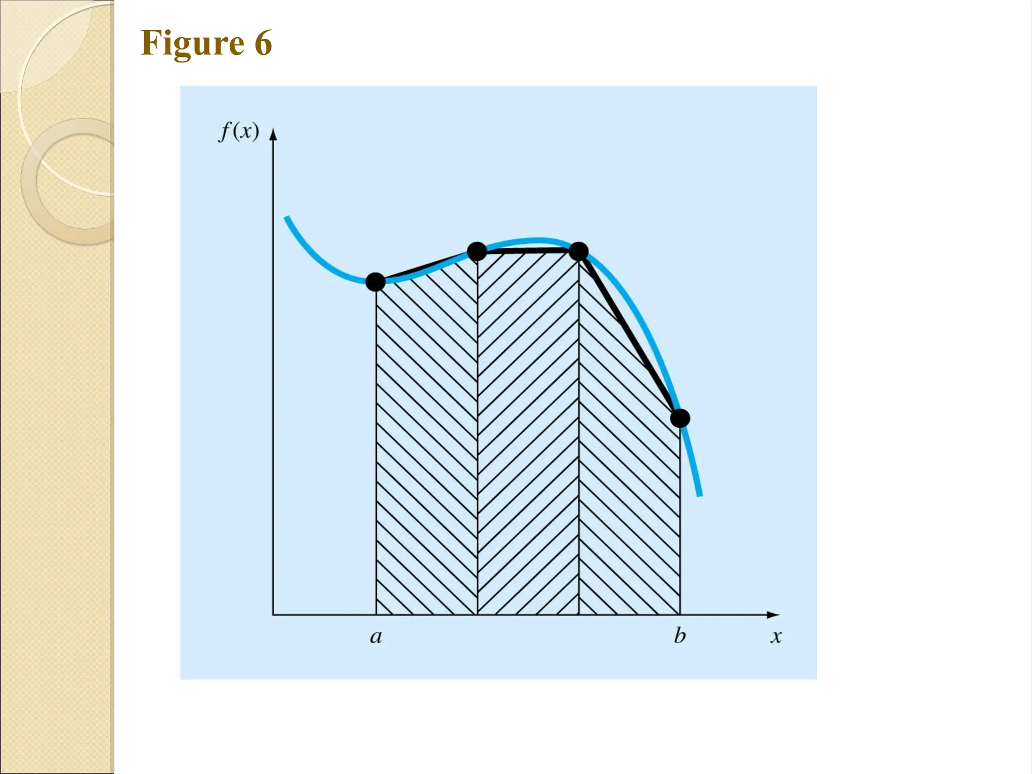
8. Copyright © 2006 The McGraw-Hill Companies, Inc. Permission required for reproduction or display.
Newton-Cotes Integration Formulas
Newton-Cotes Integration Formulas
 The Newton-Cotes formulas are the most common
numerical integration schemes.
 They are based on the strategy of replacing a
complicated function or tabulated data with an
approximating function that is easy to integrate:
n
n
n
n
n
b
a
n
b
a
x
a
x
a
x
a
a
x
f
dx
x
f
dx
x
f
I











1
1
1
0
)
(
)
(
)
(


9. Copyright © 2006 The McGraw-Hill Companies, Inc. Permission required for reproduction or display.
Figure 5

10. Copyright © 2006 The McGraw-Hill Companies, Inc. Permission required for reproduction or display.
Figure 6

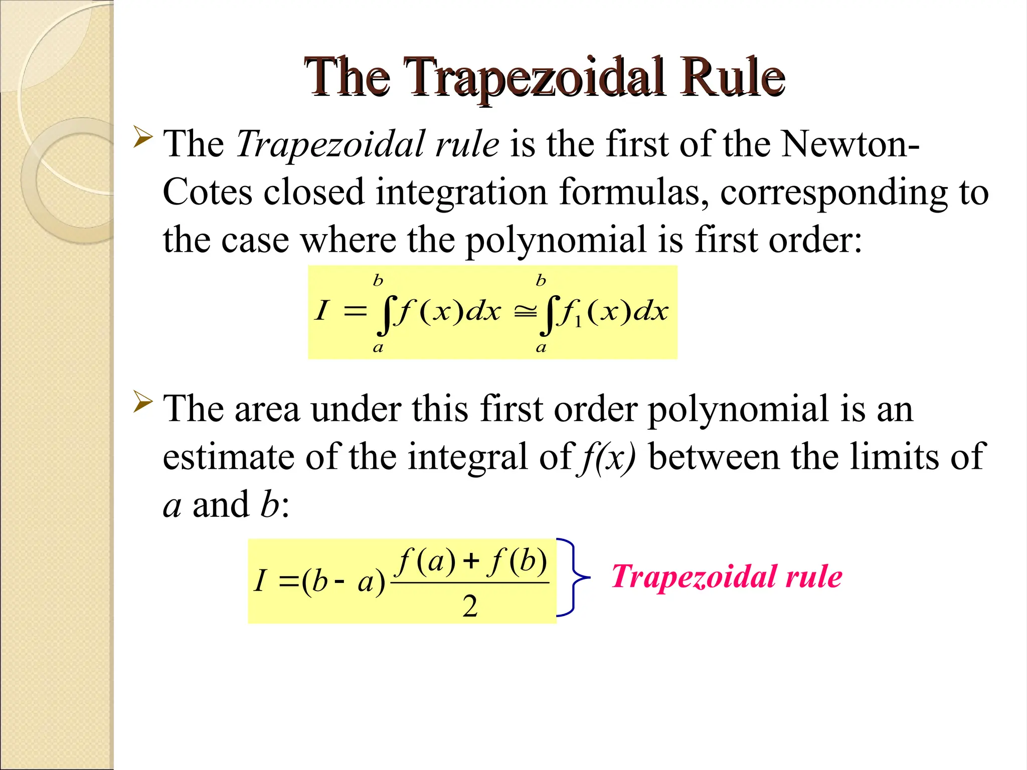
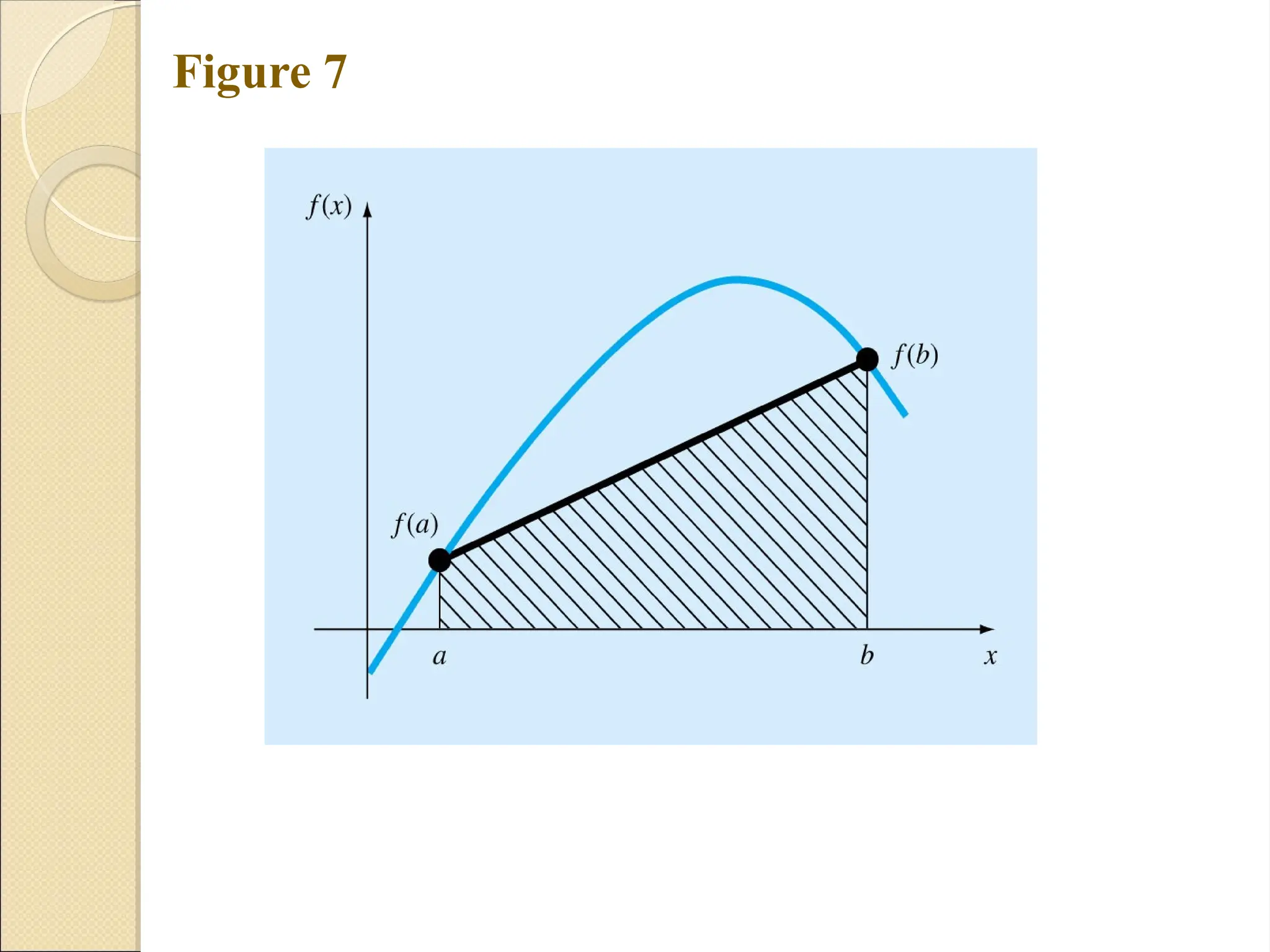
11. Copyright © 2006 The McGraw-Hill Companies, Inc. Permission required for reproduction or display.
The Trapezoidal Rule
The Trapezoidal Rule
 The Trapezoidal rule is the first of the Newton-
Cotes closed integration formulas, corresponding to
the case where the polynomial is first order:
 The area under this first order polynomial is an
estimate of the integral of f(x) between the limits of
a and b:

 

b
a
b
a
dx
x
f
dx
x
f
I )
(
)
( 1
2
)
(
)
(
)
(
b
f
a
f
a
b
I


 Trapezoidal rule

12. Copyright © 2006 The McGraw-Hill Companies, Inc. Permission required for reproduction or display.
Figure 7

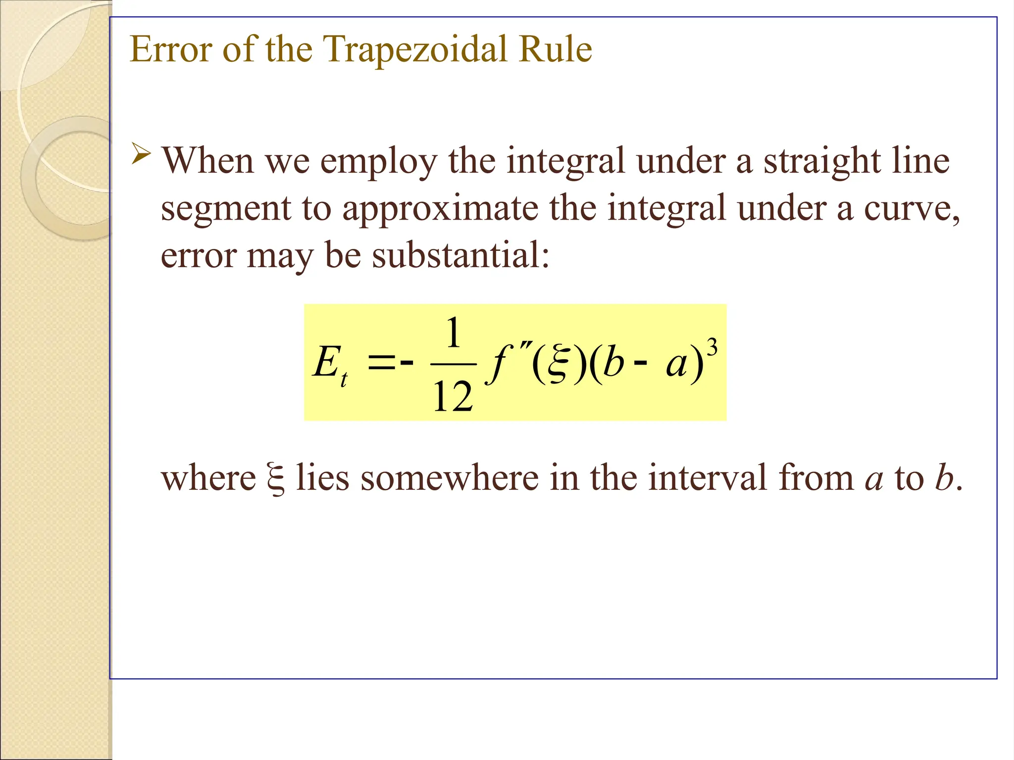
13. Copyright © 2006 The McGraw-Hill Companies, Inc. Permission required for reproduction or display.
Error of the Trapezoidal Rule
 When we employ the integral under a straight line
segment to approximate the integral under a curve,
error may be substantial:
where  lies somewhere in the interval from a to b.
3
)
)(
(
12
1
a
b
f
Et 



 

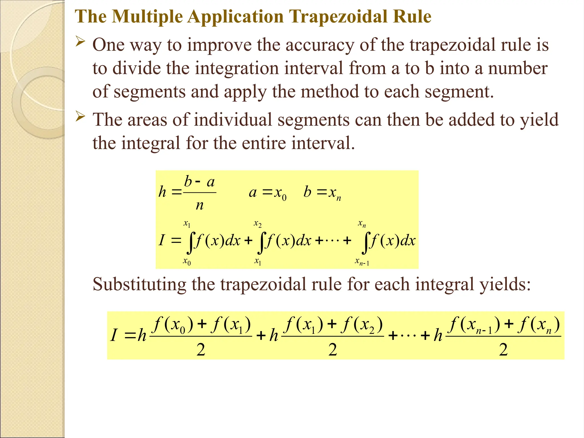
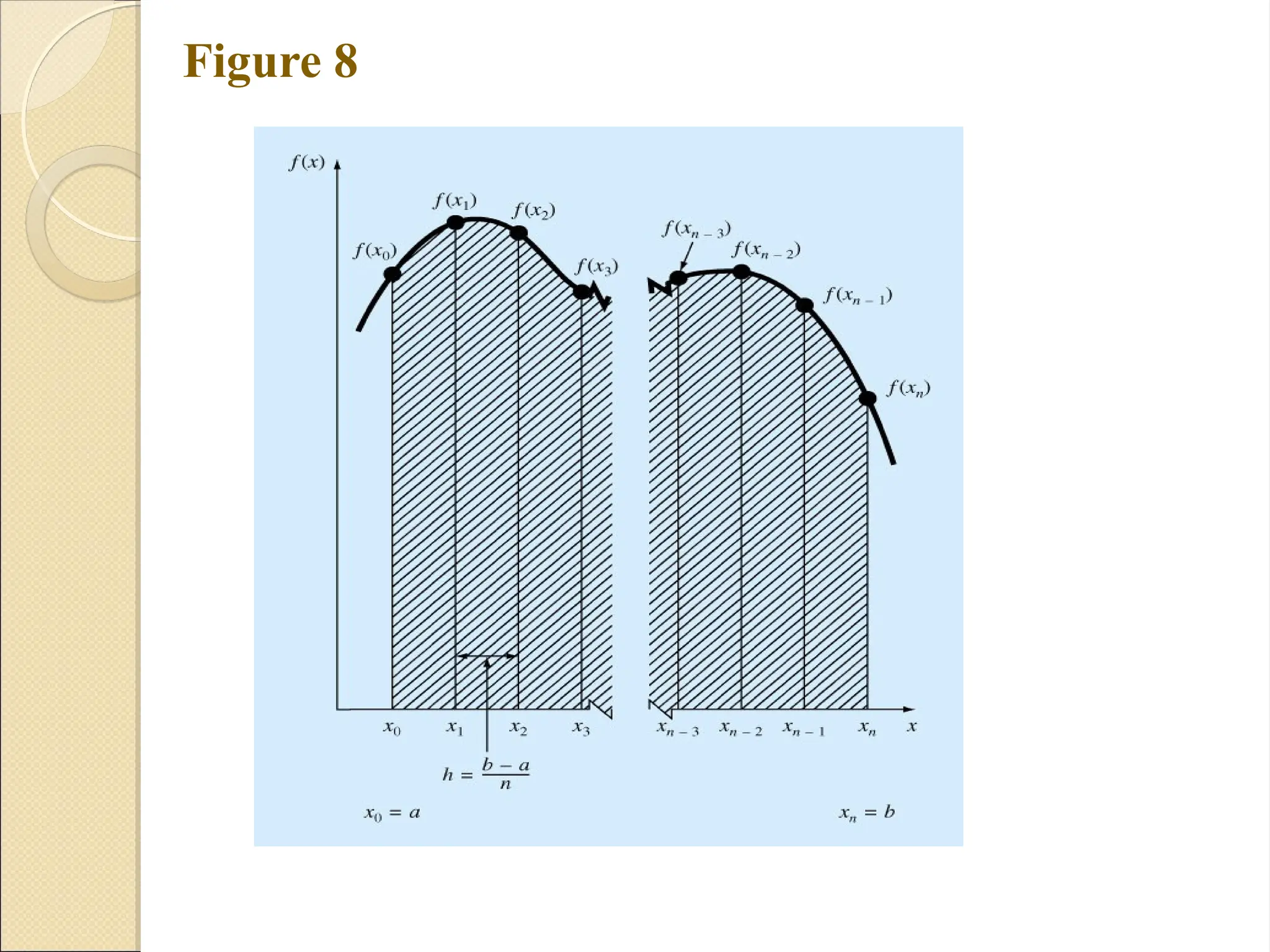
14. Copyright © 2006 The McGraw-Hill Companies, Inc. Permission required for reproduction or display.
The Multiple Application Trapezoidal Rule
 One way to improve the accuracy of the trapezoidal rule is
to divide the integration interval from a to b into a number
of segments and apply the method to each segment.
 The areas of individual segments can then be added to yield
the integral for the entire interval.
Substituting the trapezoidal rule for each integral yields:












n
n
x
x
x
x
x
x
n
dx
x
f
dx
x
f
dx
x
f
I
x
b
x
a
n
a
b
h
1
2
1
1
0
)
(
)
(
)
(
0

2
)
(
)
(
2
)
(
)
(
2
)
(
)
( 1
2
1
1
0 n
n x
f
x
f
h
x
f
x
f
h
x
f
x
f
h
I






 


15. Copyright © 2006 The McGraw-Hill Companies, Inc. Permission required for reproduction or display.
Figure 8

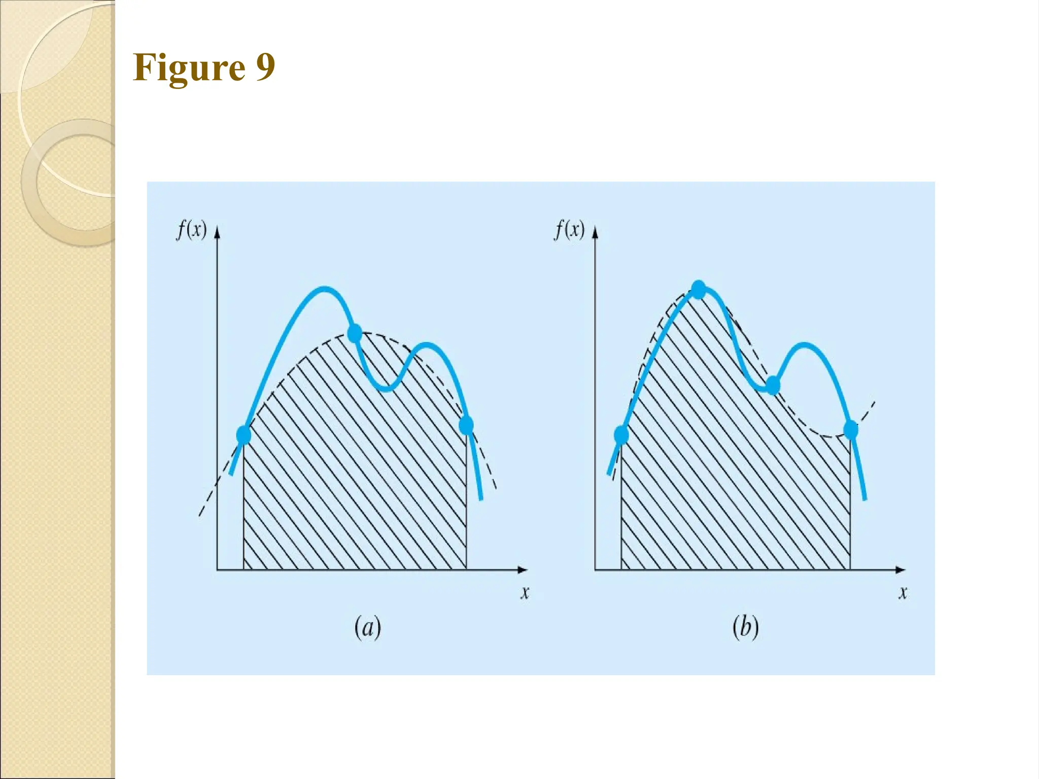
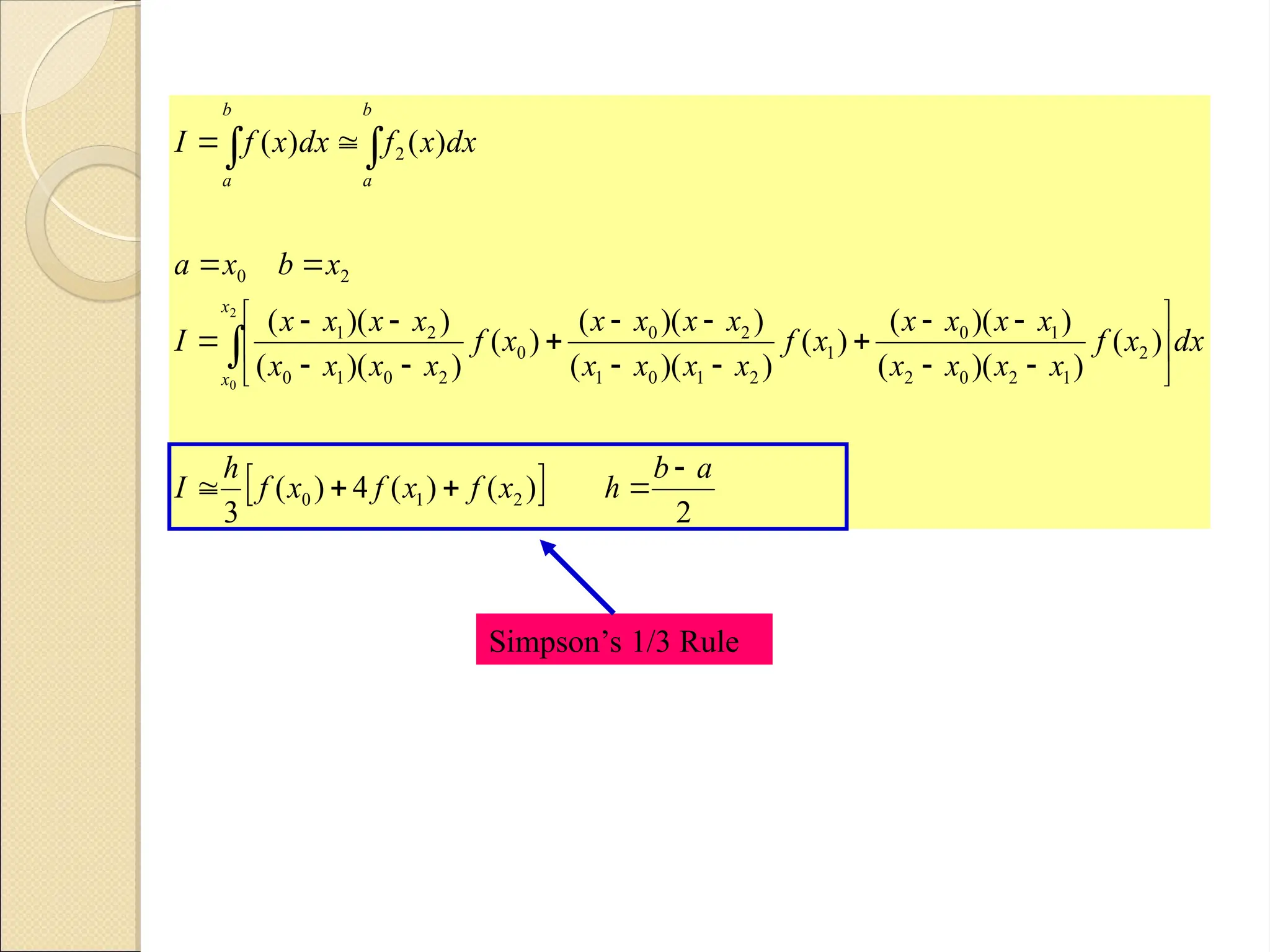
16. Copyright © 2006 The McGraw-Hill Companies, Inc. Permission required for reproduction or display.
Simpson’s Rules
Simpson’s Rules
More accurate estimate of an integral is
obtained if a high-order polynomial is used
to connect the points. The formulas that
result from taking the integrals under such
polynomials are called Simpson’s rules.
Simpson’s 1/3 Rule
Results when a second-order interpolating
polynomial is used.

17. Copyright © 2006 The McGraw-Hill Companies, Inc. Permission required for reproduction or display.
Figure 9

18. Copyright © 2006 The McGraw-Hill Companies, Inc. Permission required for reproduction or display.
 
2
)
(
)
(
4
)
(
3
)
(
)
)(
(
)
)(
(
)
(
)
)(
(
)
)(
(
)
(
)
)(
(
)
)(
(
)
(
)
(
2
1
0
2
1
2
0
2
1
0
1
2
1
0
1
2
0
0
2
0
1
0
2
1
2
0
2
2
0
a
b
h
x
f
x
f
x
f
h
I
dx
x
f
x
x
x
x
x
x
x
x
x
f
x
x
x
x
x
x
x
x
x
f
x
x
x
x
x
x
x
x
I
x
b
x
a
dx
x
f
dx
x
f
I
x
x
b
a
b
a































 
Simpson’s 1/3 Rule