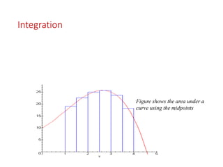
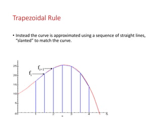
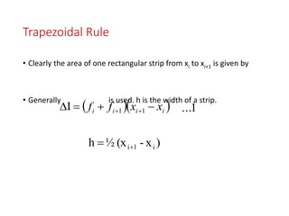
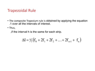
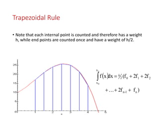
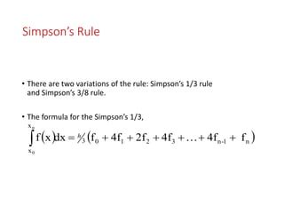
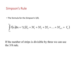
Topic : Numerical Integration & its Application.
Subject: Numerical & Statistical Methods
Name: Hemali Bishnoi (150953131003)
Dhvani Pandya (150953131011)
Shivani Saini (150953131020)
Batch : A3
Integration is an important in Physics.
Used to determine the rate of growth in bacteria or to
find the distance given the velocity (s = ∫vdt) as well as
many other uses.
The most familiar practical (probably the 1
st
usage)
use of integration is to calculate the area.
Integration
Integration
• Generally we use formulae to determine the integral of a function:
• F(x) can be found if its antiderivative, f(x) is known.
     aFbFdxxf
b
a

Integration
• when the antiderivative is unknown we are required to determine
f(x) numerically.
• To determine the definite integral we find the area between the
curve and the x-axis.
• This is the principle of numerical integration.
Integration
Figure shows the area under a
curve using the midpoints
Integration
• There are various integration methods: Trapezoid, Simpson’s, etc.
• We’ll be looking in detail at the Trapezoid and variants of the
Simpson’s method.
Trapezoidal Rule
• is an improvement on the midpoint implementation.
• the midpoints is inaccurate in that there are pieces of the “boxes”
above and below the curve (over and under estimates).
Trapezoidal Rule
• Instead the curve is approximated using a sequence of straight lines,
“slanted” to match the curve.
fi
fi+1
Trapezoidal Rule
• Clearly the area of one rectangular strip from xi to xi+1 is given by
• Generally is used. h is the width of a strip.
  iiii xxff   11I
)x-(x½h i1i
1...
Trapezoidal Rule
• The composite Trapezium rule is obtained by applying the equation
.1 over all the intervals of interest.
• Thus,
,if the interval h is the same for each strip.
 n1-n2102 f2f2f2ffI  h
Trapezoidal Rule
• Note that each internal point is counted and therefore has a weight
h, while end points are counted once and have a weight of h/2.
 
)f2f
2f2f(fdxxf
n1-n
2102
x
x
n
0

 h
Simpson’s Rule
• The midpoint rule was first improved upon by the trapezium rule.
• A further improvement is the Simpson's rule.
• Instead of approximating the curve by a straight line, we approximate
it by a quadratic or cubic function.
Simpson’s Rule
•Diagram showing approximation using Simpson’s
Rule.
Simpson’s Rule
• There are two variations of the rule: Simpson’s 1/3 rule
and Simpson’s 3/8 rule.
• The formula for the Simpson’s 1/3,
   n1-n32103
x
x
f4f4f2f4ffdxxf
n
0
 h
Simpson’s Rule
• The integration is over pairs of intervals and requires that total
number of intervals be even of the total number of points N be odd.
Simpson’s Rule
• The formula for the Simpson’s 3/8,
   n1-n32108
3
x
x
f3f2f3f3ffdxxf
n
0
 h
If the number of strips is divisible by three we can use
the 3/8 rule.
Thank You

Nsm ppt.ppt

  • 1.
    Topic : NumericalIntegration & its Application. Subject: Numerical & Statistical Methods Name: Hemali Bishnoi (150953131003) Dhvani Pandya (150953131011) Shivani Saini (150953131020) Batch : A3
  • 2.
    Integration is animportant in Physics. Used to determine the rate of growth in bacteria or to find the distance given the velocity (s = ∫vdt) as well as many other uses. The most familiar practical (probably the 1 st usage) use of integration is to calculate the area. Integration
  • 3.
    Integration • Generally weuse formulae to determine the integral of a function: • F(x) can be found if its antiderivative, f(x) is known.      aFbFdxxf b a 
  • 4.
    Integration • when theantiderivative is unknown we are required to determine f(x) numerically. • To determine the definite integral we find the area between the curve and the x-axis. • This is the principle of numerical integration.
  • 5.
    Integration Figure shows thearea under a curve using the midpoints
  • 6.
    Integration • There arevarious integration methods: Trapezoid, Simpson’s, etc. • We’ll be looking in detail at the Trapezoid and variants of the Simpson’s method.
  • 7.
    Trapezoidal Rule • isan improvement on the midpoint implementation. • the midpoints is inaccurate in that there are pieces of the “boxes” above and below the curve (over and under estimates).
  • 8.
    Trapezoidal Rule • Insteadthe curve is approximated using a sequence of straight lines, “slanted” to match the curve. fi fi+1
  • 9.
    Trapezoidal Rule • Clearlythe area of one rectangular strip from xi to xi+1 is given by • Generally is used. h is the width of a strip.   iiii xxff   11I )x-(x½h i1i 1...
  • 10.
    Trapezoidal Rule • Thecomposite Trapezium rule is obtained by applying the equation .1 over all the intervals of interest. • Thus, ,if the interval h is the same for each strip.  n1-n2102 f2f2f2ffI  h
  • 11.
    Trapezoidal Rule • Notethat each internal point is counted and therefore has a weight h, while end points are counted once and have a weight of h/2.   )f2f 2f2f(fdxxf n1-n 2102 x x n 0   h
  • 12.
    Simpson’s Rule • Themidpoint rule was first improved upon by the trapezium rule. • A further improvement is the Simpson's rule. • Instead of approximating the curve by a straight line, we approximate it by a quadratic or cubic function.
  • 13.
    Simpson’s Rule •Diagram showingapproximation using Simpson’s Rule.
  • 14.
    Simpson’s Rule • Thereare two variations of the rule: Simpson’s 1/3 rule and Simpson’s 3/8 rule. • The formula for the Simpson’s 1/3,    n1-n32103 x x f4f4f2f4ffdxxf n 0  h
  • 15.
    Simpson’s Rule • Theintegration is over pairs of intervals and requires that total number of intervals be even of the total number of points N be odd.
  • 16.
    Simpson’s Rule • Theformula for the Simpson’s 3/8,    n1-n32108 3 x x f3f2f3f3ffdxxf n 0  h If the number of strips is divisible by three we can use the 3/8 rule.
  • 17.