Downloaded 112 times

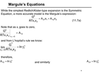
![Margule’s Equations
212121
21
E
xAxA
xRTx
G
+=
5
If you have Margule’s parameters, the activity coefficients are
easily derived from the excess Gibbs energy expression:
(11.7a)
to yield:
(11.8ab)
These empirical equations are widely used to describe binary
solutions. A knowledge of A12 and A21 at the given T is all we require
to calculate activity coefficients for a given solution composition.
]x)AA(2A[xln 1122112
2
21 −+=γ
]x)AA(2A[xln 2211221
2
12 −+=γ](https://image.slidesharecdn.com/excessgibbsfreeenergymodels-160911080126/85/Excess-gibbs-free-energy-models-5-320.jpg)

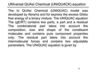

The document discusses various models for excess Gibbs free energy, primarily used in liquid-phase equilibrium calculations by engineers. It covers several empirical models, including Margules, Redlich-Kister, Van Laar, Wilson, and the Universal Quasi Chemical (Uniquac) equation, detailing their applicability and parameter dependencies. These models simplify vast experimental data into manageable equations for thermodynamic simulations, each offering specific advantages for different liquid mixture characteristics.


