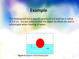
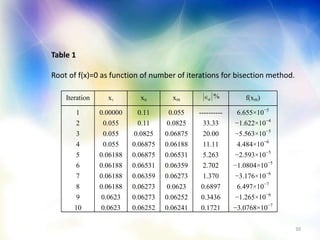
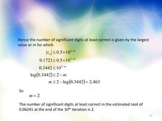
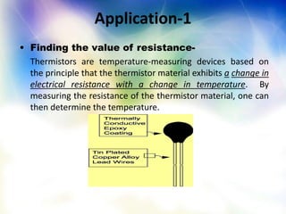
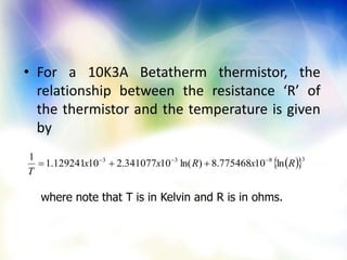
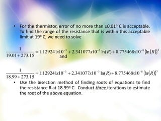
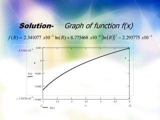
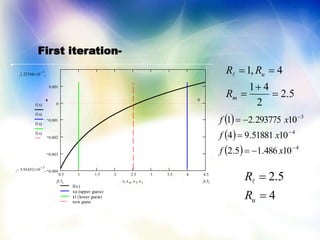
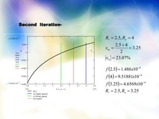
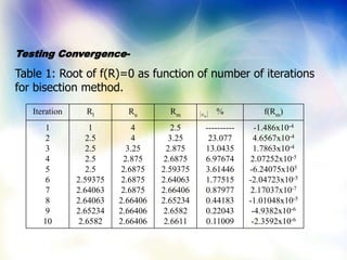
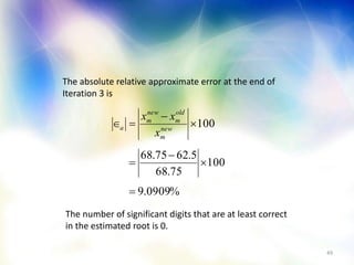
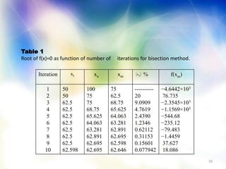
The document provides information about the bisection method for finding roots of non-linear equations. It defines the bisection method, outlines its basis and key steps, and provides an example of using the method to find the depth at which a floating ball is submerged in water. Over 10 iterations, the bisection method converges on an estimated root of 0.06241 for the example equation, with 2 significant digits found to be correct after the final iteration. The document also discusses an application of using the bisection method to find resistance of a thermistor at a given temperature.

2. Md. Rifat Rahamatulla 09.02.05.032
Md. Reduanul Islam 09.02.05.033
Md. Imran Hossain 09.02.05.035
Md. Hasibul Haque 09.02.05.036
Md. Tousif Zaman 09.02.05.038
Presented By

3. What is non-linear equation..??
• An equation in which one or more terms have a
variable of degree 2 or higher is called a nonlinear
equation. A nonlinear system of equations contains
at least one nonlinear equation.
• Non linear equation can be solved in these ways-
• 1. Bisection method.
• 2. False position method.
• 3. Newton Raphson method.
• 4. Secant method.

4. Bisection Method
a

5. Topic Outlines
• Definition.
• Basis of Bisection method.
• Steps of finding root.
• Algorithm of Bisection method.
• Example.
• Application.
• Advantage.
• Drawbacks.
• Improved method to Bisection method.
• Conclusion.

6. Definition
• The Bisection method in mathematics is a root
finding method which repeatedly bisects an
interval and then selects a subinterval in
which a root must lie for further processing.

7. Basis of Bisection Method
• Theorm 1-
An equation f(x)=0, where f(x) is a real
continuous function, has at least one root
between xl and xu if f(xl) f(xu) < 0.
x
f(x)
xu
x

8. Theorem 2- If the function f(x) in f(x)=0 changes sign between
two points, more than one root may exist between
the two points.
x
f(x)
xu
x

9. x
f(x)
xu
x
Theorem 3- If the function f(x) in f(x)=0 does not change sign
between two points, there may not be any roots
between the two points.
x
f(x)
xu
x

10. 10
Steps of finding root:
Step-1 Choose x and xu as two guesses for the root such
that f(x) f(xu) < 0, or in other words, f(x) changes sign
between x and xu. This was demonstrated in Figure 1.
x
f(x)
xu
x
Figure 1

11. x
f(x)
xu
x
xm
11
Step-2 Estimate the root, xm of the equation f (x) = 0 as the
mid point between x and xu as
x
x
m =
xu 
2
Figure 5 Estimate of xm

12. 12
Step-3 Now check the following
a) If , then the root lies between x and xm;
then x = x ; xu = xm.
b) If , then the root lies between xm and xu;
then x = xm; xu = xu.
c) If , then the root is xm. Stop the algorithm
if this is true.
    0ml xfxf
    0ml xfxf
    0ml xfxf

13. 13
x
x
m =
xu 
2
100

 new
m
old
m
new
a
x
xxm
rootofestimatecurrentnew
mx
rootofestimatepreviousold
mx
Step-4 Find the new estimate of the root
Find the absolute relative approximate error
where

14. 14
Is ?
Yes
No
Go to Step 2 using new
upper and lower guesses.
Stop the algorithm
Step-5 Compare the absolute relative approximate error with the pre-specified
error tolerance .
a
s
sa 
Note one should also check whether the number of iterations is more than the
maximum number of iterations allowed. If so, one needs to terminate the algorithm
and notify the user about it.

15. Algorithm of Bisection Method

16. 16
Example
The floating ball has a specific gravity of 0.6 and has a radius
of 5.5 cm. we are asked to find the depth to which the ball is
submerged when floating in water.
Figure 6 Diagram of the floating ball

17. 17
The equation that gives the depth x to which the ball is
submerged under water is given by
a) Use the bisection method of finding roots of equations to find
the depth x to which the ball is submerged under water.
Conduct three iterations to estimate the root of the above
equation.
b) Find the absolute relative approximate error at the end of
each iteration, and the number of significant digits at least
correct at the end of each iteration.
010993.3165.0 423
 
xx

18. 18
From the physics of the problem, the ball would be submerged
between x = 0 and x = 2R,
where R = radius of the ball,
that is
 
11.00
055.020
20



x
x
Rx
Figure 6 Diagram of the floating ball

19. To aid in the understanding of how this
method works to find the root of an
equation, the graph of f(x) is shown to the
right,
where
19
  423
1099331650 -
.x.xxf 
Figure 7 Graph of the function f(x)
Solution-

20. 20
Let us assume
11.0
00.0


ux
x
Check if the function changes sign between x and xu .
       
        4423
4423
10662.210993.311.0165.011.011.0
10993.310993.30165.000




fxf
fxf
u
l
Hence
           010662.210993.311.00 44
 
ffxfxf ul
So there is at least on root between x and xu, that is between 0 and 0.11

21. 21
Figure 8 Graph demonstrating sign change between initial limits

22. 22
055.0
2
11.00
2




 u
m
xx
x 
       
           010655.610993.3055.00
10655.610993.3055.0165.0055.0055.0
54
5423




ffxfxf
fxf
ml
m
Iteration 1
The estimate of the root is
Hence the root is bracketed between xm and xu, that is, between 0.055 and
0.11. So, the lower and upper limits of the new bracket are
At this point, the absolute relative approximate error cannot be
calculated as we do not have a previous approximation.
11.0,055.0  ul xx
a

23. 23
Figure 9 Estimate of the root for Iteration 1

24. 24
0825.0
2
11.0055.0
2




 u
m
xx
x 
       
         010655.610622.1)0825.0(055.0
10622.110993.30825.0165.00825.00825.0
54
4423




ffxfxf
fxf
ml
m
Iteration 2
The estimate of the root is
Hence the root is bracketed between x and xm, that is, between 0.055 and
0.0825. So, the lower and upper limits of the new bracket are
0825.0,055.0  ul xx

25. 25
Figure 10 Estimate of the root for Iteration 2

26. 26
The absolute relative approximate error at the end of Iteration 2 isa
%333.33
100
0825.0
055.00825.0
100






 new
m
old
m
new
m
a
x
xx
None of the significant digits are at least correct in the estimate root of xm =
0.0825 because the absolute relative approximate error is greater than 5%.

27. 27
06875.0
2
0825.0055.0
2




 u
m
xx
x 
       
           010563.510655.606875.0055.0
10563.510993.306875.0165.006875.006875.0
55
5423




ffxfxf
fxf
ml
m
Iteration 3
The estimate of the root is
Hence the root is bracketed between x and xm, that is, between 0.055 and
0.06875. So, the lower and upper limits of the new bracket are
06875.0,055.0  ul xx

28. 28
Figure 11 Estimate of the root for Iteration 3

29. 29
The absolute relative approximate error at the end of Iteration 3 is
a
%20
100
06875.0
0825.006875.0
100






 new
m
old
m
new
m
a
x
xx
Still none of the significant digits are at least correct in the estimated root of
the equation as the absolute relative approximate error is greater than 5%.
Seven more iterations were conducted and these iterations are shown in Table
1.

30. 30
Table 1
Root of f(x)=0 as function of number of iterations for bisection method.
Iteration x xu xm a % f(xm)
1
2
3
4
5
6
7
8
9
10
0.00000
0.055
0.055
0.055
0.06188
0.06188
0.06188
0.06188
0.0623
0.0623
0.11
0.11
0.0825
0.06875
0.06875
0.06531
0.06359
0.06273
0.06273
0.06252
0.055
0.0825
0.06875
0.06188
0.06531
0.06359
0.06273
0.0623
0.06252
0.06241
----------
33.33
20.00
11.11
5.263
2.702
1.370
0.6897
0.3436
0.1721
6.655×10−5
−1.622×10−4
−5.563×10−5
4.484×10−6
−2.593×10−5
−1.0804×10−5
−3.176×10−6
6.497×10−7
−1.265×10−6
−3.0768×10−7

31. 31
Hence the number of significant digits at least correct is given by the largest
value or m for which
 
  463.23442.0log2
23442.0log
103442.0
105.01721.0
105.0
2
2
2








m
m
m
m
m
a
2m
So
The number of significant digits at least correct in the estimated root of
0.06241 at the end of the 10th iteration is 2.

32. Application-1
• Finding the value of resistance-
Thermistors are temperature-measuring devices based on
the principle that the thermistor material exhibits a change in
electrical resistance with a change in temperature. By
measuring the resistance of the thermistor material, one can
then determine the temperature.

33. • For a 10K3A Betatherm thermistor, the
relationship between the resistance ‘R’ of
the thermistor and the temperature is given
by
where note that T is in Kelvin and R is in ohms.
  3833
ln10775468.8)ln(10341077.210129241.1
1
RxRxx
T



34. • For the thermistor, error of no more than ±0.01o C is acceptable.
To find the range of the resistance that is within this acceptable
limit at 19o C, we need to solve
and
• Use the bisection method of finding roots of equations to find
the resistance R at 18.99o C. Conduct three iterations to estimate
the root of the above equation.
  3833
ln10775468.8)ln(10341077.210129241.1
15.27301.19
1
RxRxx 


  3833
ln10775468.8)ln(10341077.210129241.1
15.27399.18
1
RxRxx 



35. Solution- Graph of function f(x)
   3383
10293775.2ln10775468.8)ln(10341077.2)( 
 xRxRxRf
1 1.5 2 2.5 3 3.5 4
0.003
0.002
0.001
0
0.001
f(x)
9.51881 10
4

2.29378 10
3

0
f x( )
41 x

36. Choose the bracket
 
  4
3
1051881.94
10293775.21
4
1






xf
xf
R
R
u

0.5 1 1.5 2 2.5 3 3.5 4 4.5
0.004
0.003
0.002
0.001
0
0.001
f(x)
xu (upper guess)
xl (lower guess)
1.22768 10
3

3.91652 10
3

0
f x( )
f x( )
f x( )
4.50.5 x x u x l
Entered function on given interval with initial upper and lower guesses

37. 5.2
2
41
4,1




m
u
R
RR
 
 
  4
4
3
10486.15.2
1051881.94
10293775.21






xf
xf
xf
4
5.2


uR
R
0.5 1 1.5 2 2.5 3 3.5 4 4.5
0.004
0.003
0.002
0.001
0
0.001
f(x)
xu (upper guess)
xl (lower guess)
new guess
1.22768 10
3

3.91652 10
3

0
f x( )
f x( )
f x( )
f x( )
4.50.5 x x u x l x r
First iteration-

38. Second iteration-
%07.23
25.3
2
45.2
4,5.2





a
m
u
x
RR
 
 
 
25.3,5.2
106569.425.3
1051881.94
10486.15.2
4
4
4







uRR
xf
xf
xf

0.5 1 1.5 2 2.5 3 3.5 4 4.5
0.004
0.003
0.002
0.001
0
0.001
f(x)
xu (upper guess)
xl (lower guess)
new guess
1.22768 10
3

3.91652 10
3

0
f x( )
f x( )
f x( )
f x( )
4.50.5 x x u x l x r

39. Third iteration-
875.2
2
25.35.2
25.3,5.2




m
u
R
RR
 
 
  4
4
4
107863.1875.2
106569.425.3
10486.15.2
%0435.13







xf
xf
xf
a
0.5 1 1.5 2 2.5 3 3.5 4 4.5
0.004
0.003
0.002
0.001
0
0.001
f(x)
xu (upper guess)
xl (lower guess)
new guess
1.22768 10
3

3.91652 10
3

0
f x( )
f x( )
f x( )
f x( )
4.50.5 x x u x l x r

40. Table 1: Root of f(R)=0 as function of number of iterations
for bisection method.
a
Iteration Rl Ru Rm % f(Rm)
1
2
3
4
5
6
7
8
9
10
1
2.5
2.5
2.5
2.5
2.59375
2.64063
2.64063
2.65234
2.6582
4
4
3.25
2.875
2.6875
2.6875
2.6875
2.66406
2.66406
2.66406
2.5
3.25
2.875
2.6875
2.59375
2.64063
2.66406
2.65234
2.6582
2.6611
----------
23.077
13.0435
6.97674
3.61446
1.77515
0.87977
0.44183
0.22043
0.11009
-1.486x10-4
4.6567x10-4
1.7863x10-4
2.07252x10-5
-6.24075x105
-2.04723x10-5
2.17037x10-7
-1.01048x10-5
-4.9382x10-6
-2.3592x10-6
Testing Convergence-

41. 41
Application-2
Profit Counting- We are working for a start-up computer assembly
company and have been asked to determine the minimum number of
computers that the shop will have to sell to make a profit.
The equation that gives the minimum number of
computers ‘x’ to be sold after considering the total costs
and the total sales is:
03500087540)f( 5.1
 xxx

42. 42
Use the bisection method of finding roots of equations to
find
 The minimum number of computers that need to be
sold to make a profit. Conduct three iterations to
estimate the root of the above equation.
 Find the absolute relative approximate error at the
end of each iteration, and
 The number of significant digits at least correct at the
end of each iteration.

43. 0 20 40 60 80 100
2 10
4
1 10
4
0
1 10
4
2 10
4
3 10
4
4 10
4
f(x)
3.5 10
4

1.25 10
4

0
f x( )
1000 x
43
  03500087540 5.1
 xxxf
Figure 8 Graph of the function f(x).

44. 44
Choose the bracket:
 
  12500100
1.539250


f
f
0 20 40 60 80 100 120
2 10
4
1 10
4
0
1 10
4
2 10
4
3 10
4
4 10
4
f(x)
xu (upper guess)
xl (lower guess)
3.5 10
4

1.74186 10
4

0
f x( )
f x( )
f x( )
1200 x x u x l
Entered function on given interval with initial upper and lower guesses
Figure 9 Checking the sign change
between the limits.
100and50  uxx
       
   0125001.5392
10050

 ffxfxf ul
There is at least one root between
and .
x
ux

45. 45
75
2
10050


mx
 
       0106442.41.5392
106442.475
3
3


ml xfxf
f
75and50  uxx
0 20 40 60 80 100 120
2 10
4
1 10
4
0
1 10
4
2 10
4
3 10
4
4 10
4
f(x)
xu (upper guess)
xl (lower guess)
new guess
3.5 10
4

1.74186 10
4

0
f x( )
f x( )
f x( )
f x( )
1200 x x u x l x r
Iteration 1
The estimate of the root is
Figure 10 Graph of the estimate of
the root after Iteration 1.
The root is bracketed between
and .
The new lower and upper limits of
the new bracket are
x
mx
At this point, the absolute relative approximate error cannot be calculated as we do
not have a previous approximation.

46. 46
5.62
2
7550


mx
 
        05.6250
735.765.62


ffxfxf
f
ml
0 20 40 60 80 100 120
2 10
4
1 10
4
0
1 10
4
2 10
4
3 10
4
4 10
4
f(x)
xu (upper guess)
xl (lower guess)
new guess
3.5 10
4

1.74186 10
4

0
f x( )
f x( )
f x( )
f x( )
1200 x x u x l x r
Iteration 2
The estimate of the root is
75and5.62  uxx
The root is bracketed between
and .
The new lower and upper limits of
the new bracket are
mx
ux
Figure 11 Graph of the estimate of
the root after Iteration 2.

47. 47
%20
100
5.62
755.62
100






 new
m
old
m
new
m
a
x
xx
The absolute relative approximate error at the end of
Iteration 2 is
The number of significant digits that are at least correct
in the estimated root is 0.

48. The root is bracketed between
and .
The new lower and upper limits of
the new bracket are
48
 
       0103545.2735.76
103545.275.68
75.68
2
755.62
3
3





ml
m
xfxf
f
x
0 20 40 60 80 100 120
2 10
4
1 10
4
0
1 10
4
2 10
4
3 10
4
4 10
4
f(x)
xu (upper guess)
xl (lower guess)
new guess
3.5 10
4

1.74186 10
4

0
f x( )
f x( )
f x( )
f x( )
1200 x x u x l x r
Iteration 3
The estimate of the root is
75.68and5.62  uxx
lx
mx
Figure 12 Graph of the estimate of
the root after Iteration 3.

49. 49
%0909.9
100
75.68
5.6275.68
100






 new
m
old
m
new
m
a
x
xx
The absolute relative approximate error at the end of
Iteration 3 is
The number of significant digits that are at least correct
in the estimated root is 0.

50. 50
Table 1
Root of f(x)=0 as function of number of iterations for bisection method.
aIteration xl xu xm % f(xm)
1
2
3
4
5
6
7
8
9
10
50
50
62.5
62.5
62.5
62.5
62.5
62.5
62.5
62.598
100
75
75
68.75
65.625
64.063
63.281
62.891
62.695
62.695
75
62.5
68.75
65.625
64.063
63.281
62.891
62.695
62.598
62.646
----------
20
9.0909
4.7619
2.4390
1.2346
0.62112
0.31153
0.15601
0.077942
−4.6442×103
76.735
−2.3545×103
−1.1569×103
−544.68
−235.12
−79.483
−1.4459
37.627
18.086

51. Advantage of Bisection method-
• It is a very simple method to understand.
• The bisection method is always convergent.
Since the method brackets the root, the
method is guaranteed to converge.
• Since we are halving the interval in each step,
so the method converges to the true root in a
predictable way.
51

52. • Since the method discards 50% of the interval
at each step it brackets the root in much more
quickly than the incremental search method
does. For example –
*Assuming a root is somewhere in the interval
between 0 and 1, it takes 6-7 function
evaluations to estimate the root within 0.1
accuracy.
*Those same 6-7 function evaluations using
bisecting estimate the root within 0.031
accuracy.
52

53. 5353
Drawbacks
 It may take many iterations.
 If one of the initial guesses is close to the
root, the convergence is slower.
 The method can not find complex roots of
polynomials
The bisection method only finds root when
the function crosses the x axis.

54. 54
• If a function f(x) is such that it just touches
the x-axis it will be unable to find the lower
and upper guesses.
f(x)
x
  2
xxf 

55. 55
 Function changes sign but root does not exist
f(x)
x
 
x
xf
1


56. Improved method to Bisection method-
• Regula Falsi Method: Regula Falsi method (false
position) is a root-finding method based on linear
interpolation. Its convergence is linear, but it is usually faster
than bisection
• Newton Raphson method: This method works faster
than the Bisection method and also much more accurate.
• Brent Method: Brent method combines an interpolation
strategy with the bisection algorithm. On each iteration, Brent
method approximates the function using an interpolating
curve.

57. Conclusion
This bisection method is a very simple and a robust
method and it is one of the first numerical methods
developed to find root of a non-linear equation .But
at the same time it is relatively very slow method.
We can use this method for various purpose related
to non linear continuous functions. Though it is a
slow one ,but it is one of the most reliable methods
for finding the root of a non-linear equation.