Downloaded 138 times
![Gaussian Quadratures
• Newton-Cotes Formulae
– use evenly-spaced functional values
– Did not use the flexibility we have to select the quadrature points
• In fact a quadrature point has several degrees of freedom.
Q(f)=∑i=1m ci f(xi)
A formula with m function evaluations requires specification of
2m numbers ci and xi
• Gaussian Quadratures
– select both these weights and locations so that a higher order
polynomial can be integrated (alternatively the error is proportional
to a higher derivatives)
• Price: functional values must now be evaluated at nonuniformly distributed points to achieve higher accuracy
• Weights are no longer simple numbers
• Usually derived for an interval such as [-1,1]
• Other intervals [a,b] determined by mapping to [-1,1]](https://image.slidesharecdn.com/gaussianquadratures-140128182651-phpapp01/85/Gaussian-quadratures-1-320.jpg)
![Gaussian Quadratures
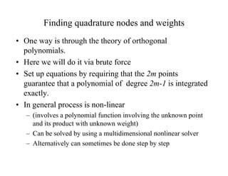
• Newton-Cotes Formulae
– use evenly-spaced functional values
– Did not use the flexibility we have to select the quadrature points
• In fact a quadrature point has several degrees of freedom.
Q(f)=∑i=1m ci f(xi)
A formula with m function evaluations requires specification of
2m numbers ci and xi
• Gaussian Quadratures
– select both these weights and locations so that a higher order
polynomial can be integrated (alternatively the error is proportional
to a higher derivatives)
• Price: functional values must now be evaluated at nonuniformly distributed points to achieve higher accuracy
• Weights are no longer simple numbers
• Usually derived for an interval such as [-1,1]
• Other intervals [a,b] determined by mapping to [-1,1]](https://image.slidesharecdn.com/gaussianquadratures-140128182651-phpapp01/75/Gaussian-quadratures-1-2048.jpg)
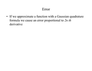
![Gaussian Quadrature on [-1, 1]
∫
1
−1
n
f ( x )dx ≈ ∑ c i f ( x i ) = c 1 f ( x 1 ) + c 2 f ( x 2 ) + L + c n f ( x n )
i =1
• Two function evaluations:
– Choose (c1, c2, x1, x2) such that the method yields “exact
integral” for f(x) = x0, x1, x2, x3
n=2:
∫
1
−1
f(x)dx
= c 1 f(x 1 ) + c 2 f(x 2 )
-1
x1
x2
1](https://image.slidesharecdn.com/gaussianquadratures-140128182651-phpapp01/85/Gaussian-quadratures-2-320.jpg)
![Gaussian Quadrature on [-1, 1]
n=2:
∫
1
−1
f(x)dx = c 1 f(x 1 ) + c 2 f(x 2 )
Exact integral for f = x0, x1, x2, x3
– Four equations for four unknowns
⎧f
⎪
⎪
⎪f
⎨
⎪f
⎪
⎪f
⎩
1
= 1 ⇒ ∫ 1dx = 2 = c 1 + c 2
−1
1
= x ⇒ ∫ xdx = 0 = c 1 x 1 + c 2 x 2
−1
2
2
2
= x ⇒ ∫ x dx = = c 1 x 1 + c 2 x 2
−1
3
2
1
2
1
3
3
= x ⇒ ∫ x 3 dx = 0 = c 1 x 1 + c 2 x 2
3
−1
1
I = ∫ f ( x )dx = f ( −
−1
⎧c 1 = 1
⎪c = 1
⎪ 2
−1
⎪
⇒ ⎨ x1 =
3
⎪
1
⎪
⎪ x2 = 3
⎩
1
3
)+ f (
1
3
)](https://image.slidesharecdn.com/gaussianquadratures-140128182651-phpapp01/85/Gaussian-quadratures-4-320.jpg)
![Gaussian Quadrature on [-1, 1]
n=3:
∫
1
−1
f ( x )dx = c 1 f ( x 1 ) + c 2 f ( x 2 ) + c 3 f ( x 3 )
x2
x3
-1 x1
1
• Choose (c1, c2, c3, x1, x2, x3) such that the method
yields “exact integral” for f(x) = x0, x1, x2, x3,x4, x5](https://image.slidesharecdn.com/gaussianquadratures-140128182651-phpapp01/85/Gaussian-quadratures-6-320.jpg)
![Gaussian Quadrature on [-1, 1]
1
f = 1 ⇒ ∫ xdx = 2 = c1 + c2 + c3
−1
1
f = x ⇒ ∫ xdx = 0 = c1 x1 + c2 x2 + c3 x3
−1
1
2
2
2
f = x ⇒ ∫ x dx = = c1 x12 + c2 x2 + c3 x3
3
−1
2
2
1
3
3
f = x 3 ⇒ ∫ x 3dx = 0 = c1 x13 + c2 x2 + c3 x3
−1
1
2
4
4
f = x ⇒ ∫ x dx = = c1 x14 + c2 x2 + c3 x3
5
−1
4
4
1
5
5
f = x 5 ⇒ ∫ x 5 dx = 0 = c1 x15 + c2 x2 + c3 x3
−1
⎧c1 = 5 / 9
⎪c = 8 / 9
⎪ 2
⎪c3 = 5 / 9
⎪
⇒⎨
⎪ x1 = − 3 / 5
⎪ x2 = 0
⎪
⎪ x3 = 3 / 5
⎩](https://image.slidesharecdn.com/gaussianquadratures-140128182651-phpapp01/85/Gaussian-quadratures-7-320.jpg)
![Gaussian Quadrature on [-1, 1]
Exact integral for f = x0, x1, x2, x3, x4, x5
I=∫
1
−1
3
5
3
8
5
)
f ( x )dx = f ( −
)+ f (0 )+ f (
9
5
9
5
9](https://image.slidesharecdn.com/gaussianquadratures-140128182651-phpapp01/85/Gaussian-quadratures-8-320.jpg)
![Gaussian Quadrature on [a, b]
Coordinate transformation from [a,b] to [-1,1]
b−a
b+a
t=
x+
2
2
⎧ x = −1 ⇒ t = a
⎨
⎩x = 1 ⇒ t = b
a
∫
b
a
t1
f ( t )dt = ∫
1
−1
t2
b
1
b−a
b+a b−a
f(
x+
)(
)dx = ∫ g ( x )dx
−1
2
2
2](https://image.slidesharecdn.com/gaussianquadratures-140128182651-phpapp01/85/Gaussian-quadratures-9-320.jpg)
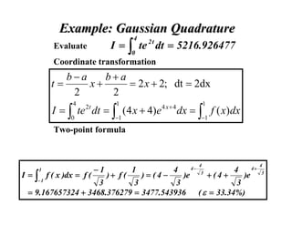
![Example: Gaussian Quadrature
Three-point formula
1
5
8
5
I = ∫ f ( x )dx = f ( − 0.6 ) + f ( 0 ) + f ( 0.6 )
−1
9
9
9
5
8
5
4 − 0 .6
4
= ( 4 − 4 0.6 )e
+ ( 4 )e + ( 4 + 4 0.6 )e 4 + 0.6
9
9
9
5
8
5
= ( 2.221191545 ) + ( 218.3926001 ) + ( 8589.142689 )
9
9
9
= 4967.106689
( ε = 4.79%)
Four-point formula
I = ∫ f ( x )dx = 0.34785[ f ( −0.861136 ) + f ( 0.861136 )]
1
−1
+ 0.652145 [ f ( −0.339981 ) + f ( 0.339981 )]
= 5197.54375
( ε = 0.37%)](https://image.slidesharecdn.com/gaussianquadratures-140128182651-phpapp01/85/Gaussian-quadratures-11-320.jpg)

This document discusses Gaussian quadrature, a method for numerical integration. It begins by comparing Gaussian quadrature to Newton-Cotes formulae, noting that Gaussian quadrature selects both weights and locations of integration points to exactly integrate higher order polynomials. The document then provides examples of 2-point and 3-point Gaussian quadrature on the interval [-1,1], showing how to determine the points and weights to integrate polynomials up to a certain order exactly. It also discusses extending Gaussian quadrature to other intervals via a coordinate transformation, and provides an example integration problem.