Download as PDF, PPTX

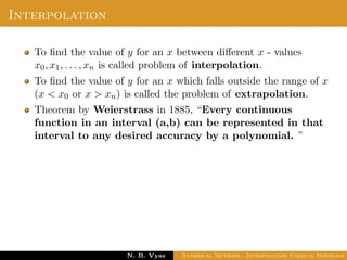

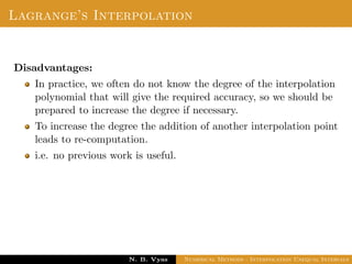
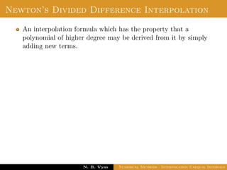
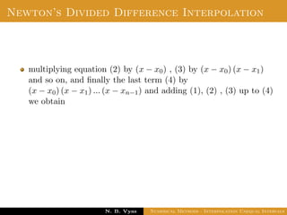


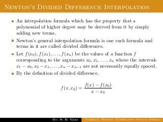
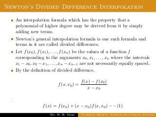
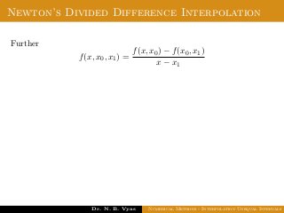
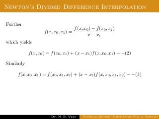
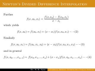
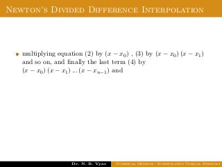
![Newton’s Divided Difference Interpolation
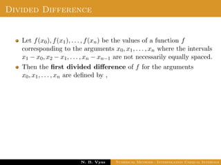
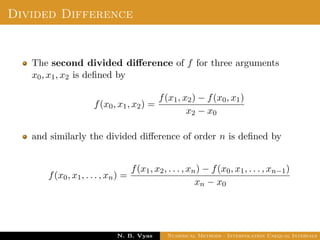
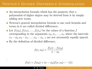
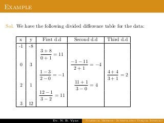
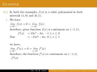
The divided difference upto third order
x y 1stdiv.diff. 2nddiv.diff. 3rddiv.diff.
x0 y0
[x0, x1]
x1 y1 [x0, x1, x2]
[x1, x2] [x0, x1, x2, x3]
x2 y2 [x1, x2, x3]
[x2, x3]
x3 y3
Dr. N. B. Vyas Numerical Methods - Interpolation Unequal Intervals](https://image.slidesharecdn.com/nm-120503065104-phpapp02/85/Interpolation-with-unequal-interval-79-320.jpg)
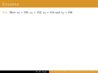
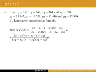
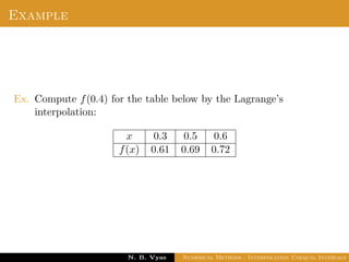
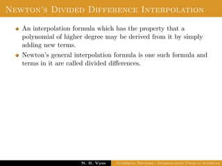
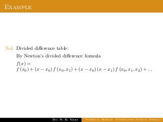
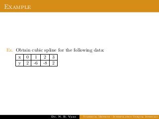
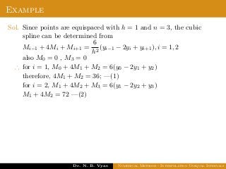
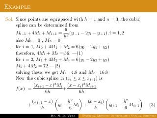
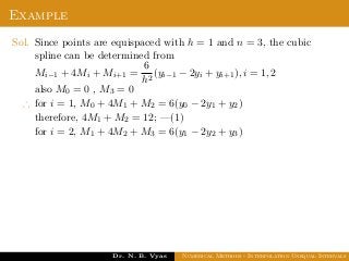
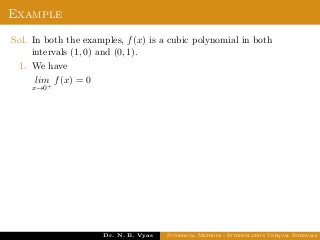
![Example
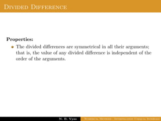
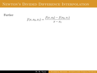
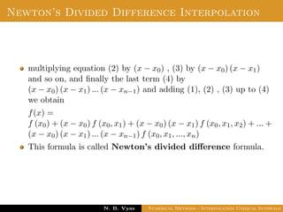
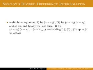
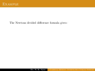
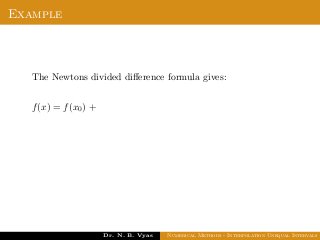
The Newtons divided difference formula gives:
f(x) = f(x0) + (x − x0)f[x0, x1] + (x − x0)(x − x1)f[x0, x1, x2]
Dr. N. B. Vyas Numerical Methods - Interpolation Unequal Intervals](https://image.slidesharecdn.com/nm-120503065104-phpapp02/85/Interpolation-with-unequal-interval-86-320.jpg)
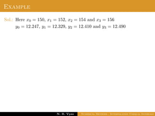
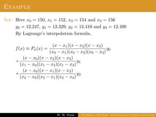
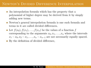
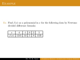
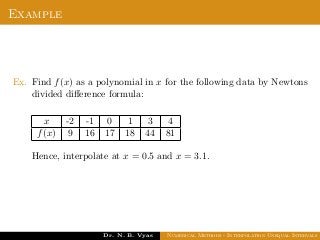
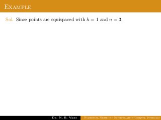
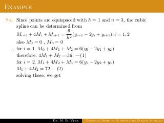
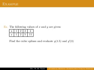
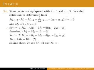
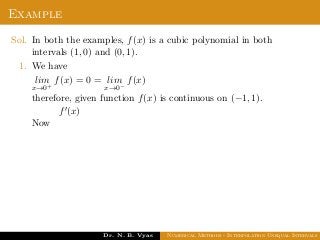
![Example
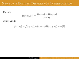
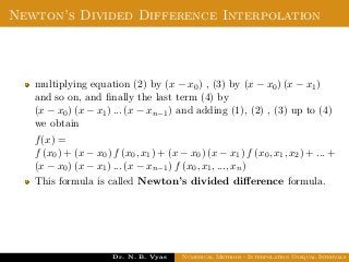
The Newtons divided difference formula gives:
f(x) = f(x0) + (x − x0)f[x0, x1] + (x − x0)(x − x1)f[x0, x1, x2]
+
Dr. N. B. Vyas Numerical Methods - Interpolation Unequal Intervals](https://image.slidesharecdn.com/nm-120503065104-phpapp02/85/Interpolation-with-unequal-interval-87-320.jpg)
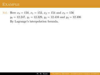
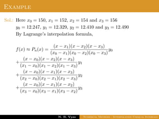
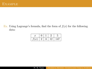
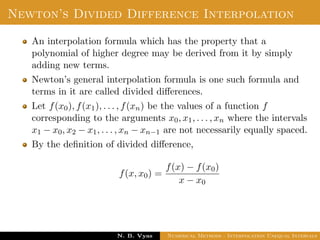
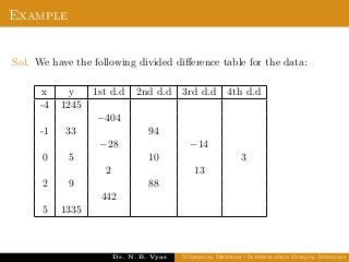
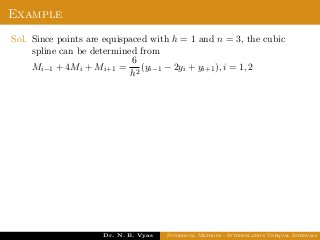
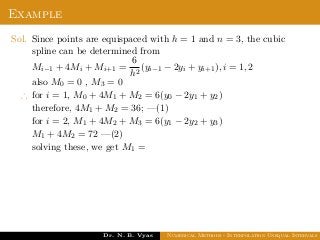
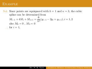
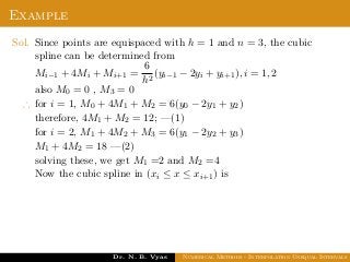
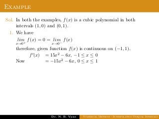
![Example
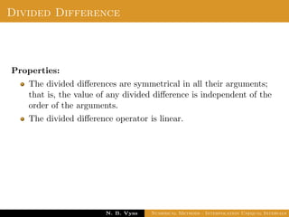
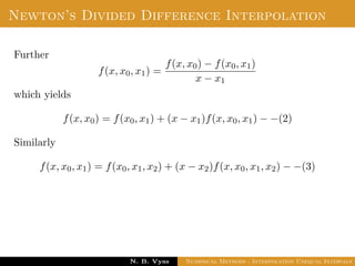
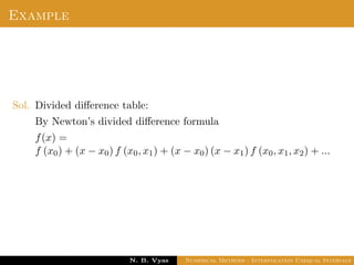
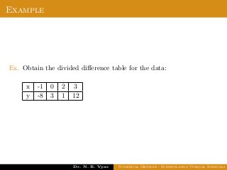
The Newtons divided difference formula gives:
f(x) = f(x0) + (x − x0)f[x0, x1] + (x − x0)(x − x1)f[x0, x1, x2]
+ (x − x0)(x − x1)(x − x2)f[x0, x1, x2, x3]
Dr. N. B. Vyas Numerical Methods - Interpolation Unequal Intervals](https://image.slidesharecdn.com/nm-120503065104-phpapp02/85/Interpolation-with-unequal-interval-88-320.jpg)
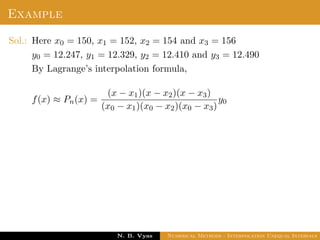
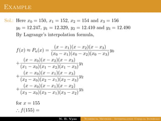
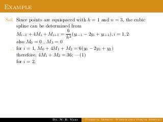
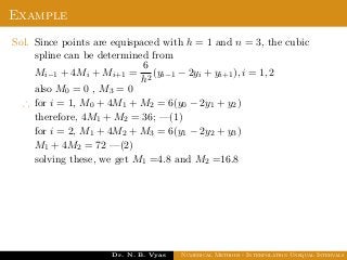
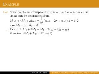
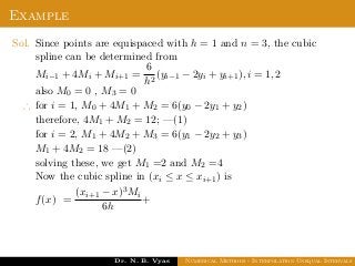
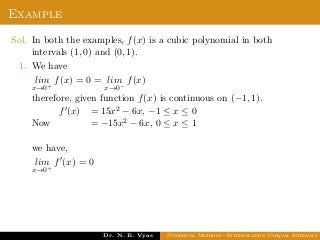
![Example
The Newtons divided difference formula gives:
f(x) = f(x0) + (x − x0)f[x0, x1] + (x − x0)(x − x1)f[x0, x1, x2]
+ (x − x0)(x − x1)(x − x2)f[x0, x1, x2, x3]
+
Dr. N. B. Vyas Numerical Methods - Interpolation Unequal Intervals](https://image.slidesharecdn.com/nm-120503065104-phpapp02/85/Interpolation-with-unequal-interval-89-320.jpg)
![Example
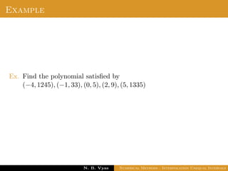
The Newtons divided difference formula gives:
f(x) = f(x0) + (x − x0)f[x0, x1] + (x − x0)(x − x1)f[x0, x1, x2]
+ (x − x0)(x − x1)(x − x2)f[x0, x1, x2, x3]
+ (x − x0)(x − x1)(x − x2)(x − x3)f[x0, x1, x2, x3, x4]
Dr. N. B. Vyas Numerical Methods - Interpolation Unequal Intervals](https://image.slidesharecdn.com/nm-120503065104-phpapp02/85/Interpolation-with-unequal-interval-90-320.jpg)
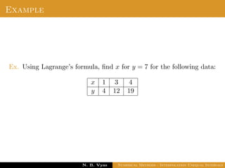
![Example
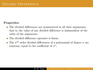
The Newtons divided difference formula gives:
f(x) = f(x0) + (x − x0)f[x0, x1] + (x − x0)(x − x1)f[x0, x1, x2]
+ (x − x0)(x − x1)(x − x2)f[x0, x1, x2, x3]
+ (x − x0)(x − x1)(x − x2)(x − x3)f[x0, x1, x2, x3, x4]
= ...
= 3x4 − 5x3 + 6x2 − 14x + 5
Dr. N. B. Vyas Numerical Methods - Interpolation Unequal Intervals](https://image.slidesharecdn.com/nm-120503065104-phpapp02/85/Interpolation-with-unequal-interval-91-320.jpg)
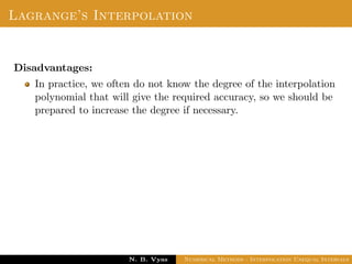
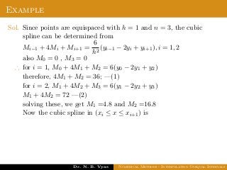
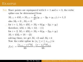
![Example
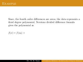
Since, the fourth order differences are zeros, the data represents a
third degree polynomial. Newtons divided difference formula
gives the polynomial as
f(x) = f(x0) + (x − x0)f[x0, x1] + (x − x0)(x − x1)f[x0, x1, x2]
Dr. N. B. Vyas Numerical Methods - Interpolation Unequal Intervals](https://image.slidesharecdn.com/nm-120503065104-phpapp02/85/Interpolation-with-unequal-interval-95-320.jpg)
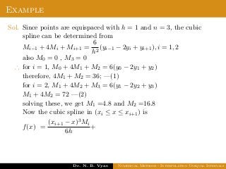
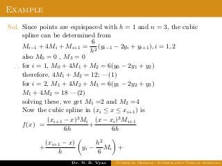
![Example
Since, the fourth order differences are zeros, the data represents a
third degree polynomial. Newtons divided difference formula
gives the polynomial as
f(x) = f(x0) + (x − x0)f[x0, x1] + (x − x0)(x − x1)f[x0, x1, x2]
+
Dr. N. B. Vyas Numerical Methods - Interpolation Unequal Intervals](https://image.slidesharecdn.com/nm-120503065104-phpapp02/85/Interpolation-with-unequal-interval-96-320.jpg)
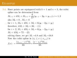
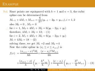
![Example
Since, the fourth order differences are zeros, the data represents a
third degree polynomial. Newtons divided difference formula
gives the polynomial as
f(x) = f(x0) + (x − x0)f[x0, x1] + (x − x0)(x − x1)f[x0, x1, x2]
+ (x − x0)(x − x1)(x − x2)f[x0, x1, x2, x3]
Dr. N. B. Vyas Numerical Methods - Interpolation Unequal Intervals](https://image.slidesharecdn.com/nm-120503065104-phpapp02/85/Interpolation-with-unequal-interval-97-320.jpg)
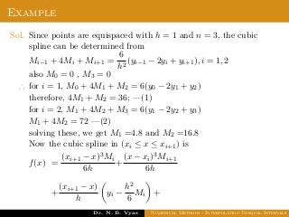
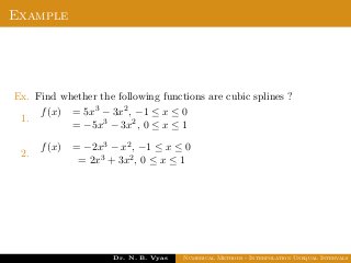
![Example
Since, the fourth order differences are zeros, the data represents a
third degree polynomial. Newtons divided difference formula
gives the polynomial as
f(x) = f(x0) + (x − x0)f[x0, x1] + (x − x0)(x − x1)f[x0, x1, x2]
+ (x − x0)(x − x1)(x − x2)f[x0, x1, x2, x3]
= ...
= x3 + 17
Dr. N. B. Vyas Numerical Methods - Interpolation Unequal Intervals](https://image.slidesharecdn.com/nm-120503065104-phpapp02/85/Interpolation-with-unequal-interval-98-320.jpg)


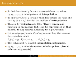
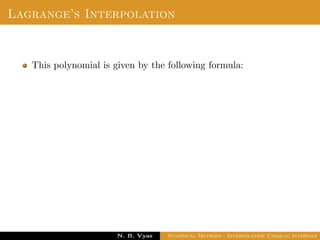
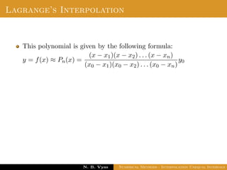
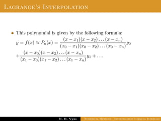
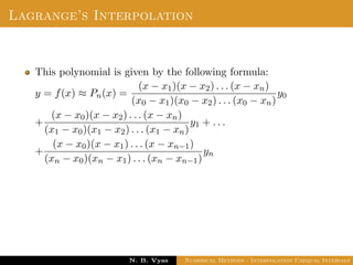
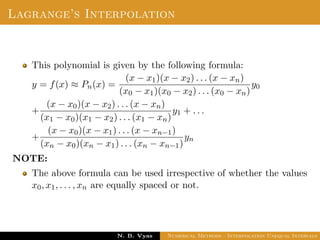
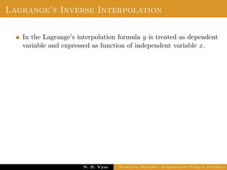
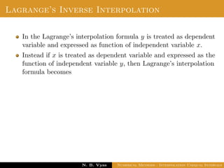
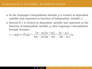
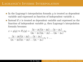
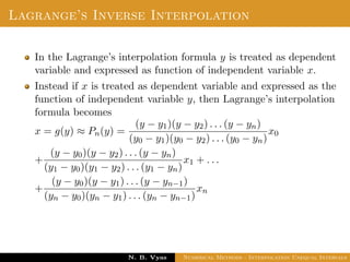
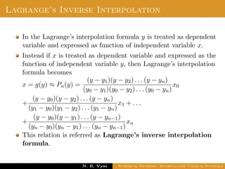
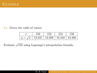
The document discusses numerical methods for interpolation with unequal intervals, focusing on Lagrange's interpolation formula, which allows for determining the value of y for a given x when data points are not evenly spaced. It explains the concepts of interpolation and extrapolation, the Weierstrass theorem about polynomial representation of continuous functions, and includes an example demonstrating the application of Lagrange’s interpolation in evaluating square roots. Furthermore, it introduces Lagrange's inverse interpolation, adapting the formula to find x as a function of y.