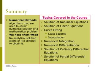
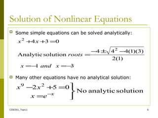
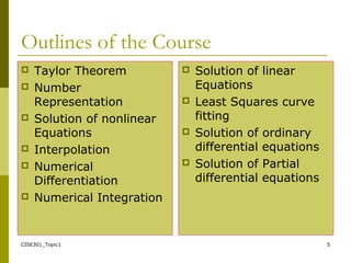
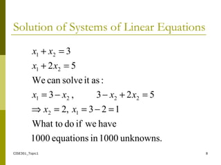
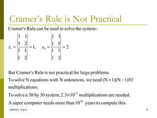
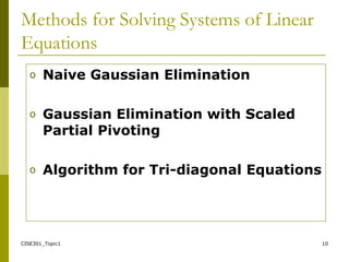
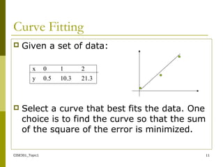
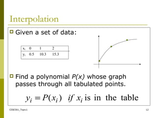
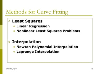
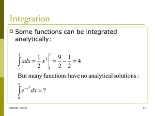
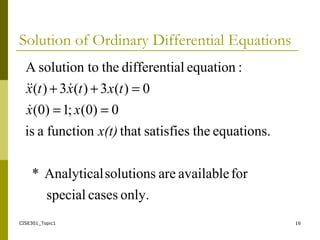
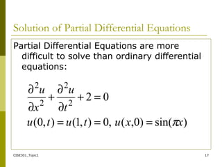
This document provides an overview of the topics covered in the Numerical Methods course CISE-301. It discusses: - Numerical methods as algorithms used to obtain numerical solutions to mathematical problems when analytical solutions do not exist or are difficult to obtain. - Specific topics that will be covered, including solution of nonlinear equations, linear equations, curve fitting, interpolation, numerical integration, differentiation, and ordinary and partial differential equations. 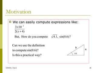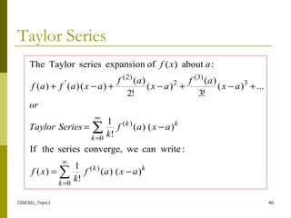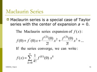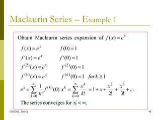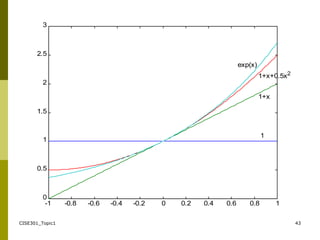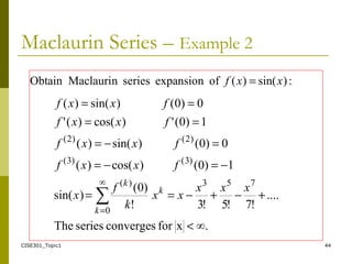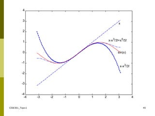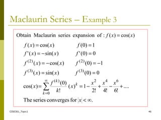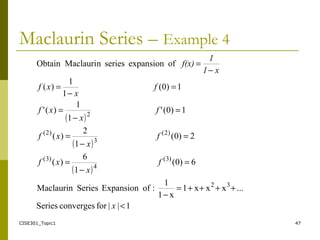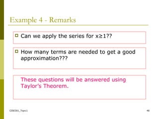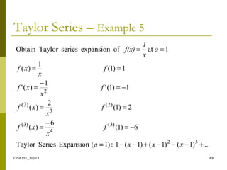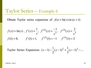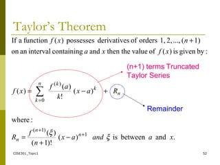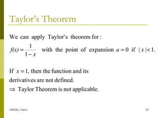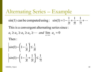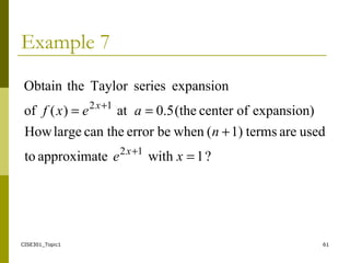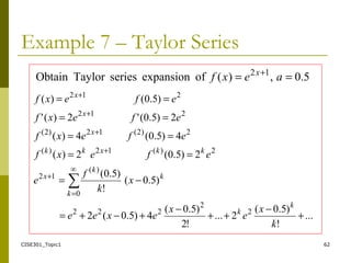- An introduction to Taylor series and how they can be used to approximate functions, along with examples of Maclaurin series expansions. 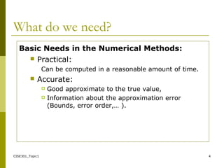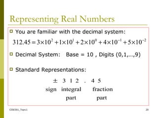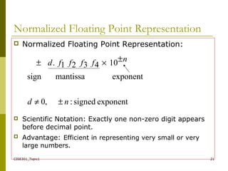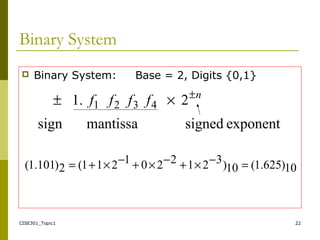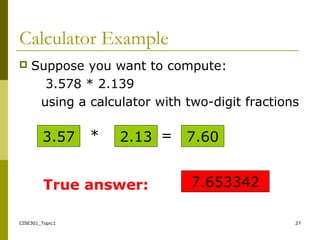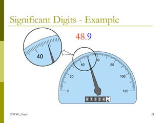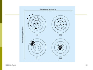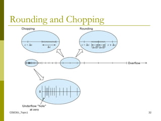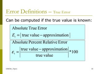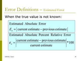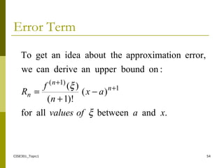- How numerical representations of real numbers like floating point can lead to rounding errors, and the concepts of accuracy and precision in numerical calculations.

1. CISE301_Topic1 1
CISE-301: Numerical Methods
Topic 1:
Introduction to Numerical Methods and Taylor Series
Lectures 1-4:

2. CISE301_Topic1 2
Lecture 1
Introduction to Numerical Methods
 What are NUMERICAL METHODS?
 Why do we need them?
 Topics covered in CISE301.
Reading Assignment: Pages 3-10 of textbook

3. CISE301_Topic1 3
Numerical Methods
Numerical Methods:
Algorithms that are used to obtain numerical
solutions of a mathematical problem.
Why do we need them?
1. No analytical solution exists,
2. An analytical solution is difficult to obtain
or not practical.

4. CISE301_Topic1 4
What do we need?
Basic Needs in the Numerical Methods:
 Practical:
Can be computed in a reasonable amount of time.
 Accurate:
 Good approximate to the true value,
 Information about the approximation error
(Bounds, error order,… ).

5. CISE301_Topic1 5
Outlines of the Course
 Taylor Theorem
 Number
Representation
 Solution of nonlinear
Equations
 Interpolation
 Numerical
Differentiation
 Numerical Integration
 Solution of linear
Equations
 Least Squares curve
fitting
 Solution of ordinary
differential equations
 Solution of Partial
differential equations

6. CISE301_Topic1 6
Solution of Nonlinear Equations
 Some simple equations can be solved analytically:
 Many other equations have no analytical solution:
31
)1(2
)3)(1(444
solutionAnalytic
034
2
2
−=−=
−±−
=
=++
xandx
roots
xx
solutionanalyticNo
052 29




=
=+−
−x
ex
xx

7. CISE301_Topic1 7
Methods for Solving Nonlinear Equations
o Bisection Method
o Newton-Raphson Method
o Secant Method

8. CISE301_Topic1 8
Solution of Systems of Linear Equations
unknowns.1000inequations1000
haveweifdoWhat to
123,2
523,3
:asitsolvecanWe
52
3
12
2221
21
21
=−==⇒
=+−−=
=+
=+
xx
xxxx
xx
xx

9. CISE301_Topic1 9
Cramer’s Rule is Not Practical
this.computetoyears10thanmoreneedscomputersuperA
needed.aretionsmultiplica102.3system,30by30asolveTo
tions.multiplica
1)N!1)(N(Nneedweunknowns,NwithequationsNsolveTo
problems.largeforpracticalnotisRulesCramer'But
2
21
11
51
31
,1
21
11
25
13
:systemthesolvetousedbecanRulesCramer'
20
35
21
×
−+
==== xx

10. CISE301_Topic1 10
Methods for Solving Systems of Linear
Equations
o Naive Gaussian Elimination
o Gaussian Elimination with Scaled
Partial Pivoting
o Algorithm for Tri-diagonal Equations

11. CISE301_Topic1 11
Curve Fitting
 Given a set of data:
 Select a curve that best fits the data. One
choice is to find the curve so that the sum
of the square of the error is minimized.
x 0 1 2
y 0.5 10.3 21.3

12. CISE301_Topic1 12
Interpolation
 Given a set of data:
 Find a polynomial P(x) whose graph
passes through all tabulated points.
xi 0 1 2
yi 0.5 10.3 15.3
tablein theis)( iii xifxPy =

13. CISE301_Topic1 13
Methods for Curve Fitting
o Least Squares
o Linear Regression
o Nonlinear Least Squares Problems
o Interpolation
o Newton Polynomial Interpolation
o Lagrange Interpolation

14. CISE301_Topic1 14
Integration
 Some functions can be integrated
analytically:
?
:solutionsanalyticalnohavefunctionsmanyBut
4
2
1
2
9
2
1
0
3
1
2
3
1
2
=
=−==
∫
∫
−
dxe
xxdx
a
x

15. CISE301_Topic1 15
Methods for Numerical Integration
o Upper and Lower Sums
o Trapezoid Method
o Romberg Method
o Gauss Quadrature

16. CISE301_Topic1 16
Solution of Ordinary Differential Equations
only.casesspecial
foravailablearesolutionsAnalytical*
equations.thesatisfiesthatfunctionais
0)0(;1)0(
0)(3)(3)(
:equationaldifferentitheosolution tA
x(t)
xx
txtxtx
==
=++



17. CISE301_Topic1 17
Solution of Partial Differential Equations
Partial Differential Equations are more
difficult to solve than ordinary differential
equations:
)sin()0,(,0),1(),0(
022
2
2
2
xxututu
t
u
x
u
π===
=+
∂
∂
+
∂
∂

18. CISE301_Topic1 18
Summary
 Numerical Methods:
Algorithms that are
used to obtain
numerical solution of a
mathematical problem.
 We need them when
No analytical solution
exists or it is difficult
to obtain it.
 Solution of Nonlinear Equations
 Solution of Linear Equations
 Curve Fitting
 Least Squares
 Interpolation
 Numerical Integration
 Numerical Differentiation
 Solution of Ordinary Differential
Equations
 Solution of Partial Differential
Equations
Topics Covered in the Course

19. CISE301_Topic1 19
 Number Representation
 Normalized Floating Point Representation
 Significant Digits
 Accuracy and Precision
 Rounding and Chopping
Reading Assignment: Chapter 3
Lecture 2
Number Representation and Accuracy

20. CISE301_Topic1 20
Representing Real Numbers
 You are familiar with the decimal system:
 Decimal System: Base = 10 , Digits (0,1,…,9)
 Standard Representations:
21012
10510410210110345.312 −−
×+×+×+×+×=
partpart
fractionintegralsign
54.213±

21. CISE301_Topic1 21
Normalized Floating Point Representation
 Normalized Floating Point Representation:
 Scientific Notation: Exactly one non-zero digit appears
before decimal point.
 Advantage: Efficient in representing very small or very
large numbers.
exponentsigned:,0
exponentmantissasign
104321.
nd
nffffd
±≠
±×±

22. CISE301_Topic1 22
Binary System
 Binary System: Base = 2, Digits {0,1}
exponentsignedmantissasign
2.1 4321
n
ffff ±
×±
10)625.1(10)3212201211(2)101.1( =−×+−×+−×+=

23. CISE301_Topic1 23
Fact
 Numbers that have a finite expansion in one numbering
system may have an infinite expansion in another
numbering system:
 You can never represent 1.1 exactly in binary system.
210 ...)011000001100110.1()1.1( =

24. IEEE 754 Floating-Point Standard
 Single Precision (32-bit representation)
 1-bit Sign + 8-bit Exponent + 23-bit Fraction
 Double Precision (64-bit representation)
 1-bit Sign + 11-bit Exponent + 52-bit Fraction
CISE301_Topic1 24
S Exponent8
Fraction23
S Exponent11
Fraction52
(continued)

25. CISE301_Topic1 25
Significant Digits
 Significant digits are those digits that can be
used with confidence.
 Single-Precision: 7 Significant Digits
1.175494… × 10-38
to 3.402823… × 1038
 Double-Precision: 15 Significant Digits
2.2250738… × 10-308
to 1.7976931… × 10308

26. CISE301_Topic1 26
Remarks
 Numbers that can be exactly represented are called
machine numbers.
 Difference between machine numbers is not uniform
 Sum of machine numbers is not necessarily a machine
number

27. CISE301_Topic1 27
Calculator Example
 Suppose you want to compute:
3.578 * 2.139
using a calculator with two-digit fractions
3.57 * 2.13 7.60=
7.653342True answer:

28. CISE301_Topic1 28
48.9
Significant Digits - Example

29. CISE301_Topic1 29
Accuracy and Precision
 Accuracy is related to the closeness to the true
value.
 Precision is related to the closeness to other
estimated values.

30. CISE301_Topic1 30

31. CISE301_Topic1 31
Rounding and Chopping
 Rounding: Replace the number by the nearest
machine number.
 Chopping: Throw all extra digits.

32. CISE301_Topic1 32
Rounding and Chopping

33. CISE301_Topic1 33
Can be computed if the true value is known:
100*
valuetrue
ionapproximatvaluetrue
ErrorRelativePercentAbsolute
ionapproximatvaluetrue
ErrorTrueAbsolute
t
−
=
−=
ε
tE
Error Definitions – True Error

34. CISE301_Topic1 34
When the true value is not known:
100*
estimatecurrent
estimatepreviousestimatecurrent
ErrorRelativePercentAbsoluteEstimated
estimatepreviousestimatecurrent
ErrorAbsoluteEstimated
−
=
−=
a
aE
ε
Error Definitions – Estimated Error

35. CISE301_Topic1 35
We say that the estimate is correct to n
decimal digits if:
We say that the estimate is correct to n
decimal digits rounded if:
n−
≤10Error
n−
×≤ 10
2
1
Error
Notation

36. CISE301_Topic1 36
Summary
 Number Representation
Numbers that have a finite expansion in one numbering system
may have an infinite expansion in another numbering system.
 Normalized Floating Point Representation
 Efficient in representing very small or very large numbers,
 Difference between machine numbers is not uniform,
 Representation error depends on the number of bits used in
the mantissa.

37. CISE301_Topic1 37
Lectures 3-4
Taylor Theorem
 Motivation
 Taylor Theorem
 Examples
Reading assignment: Chapter 4

38. CISE301_Topic1 38
Motivation
 We can easily compute expressions like:
?)6.0sin(,4.1computeyoudoHowBut,
)4(2
103 2
+
×
x
way?practicalathisIs
sin(0.6)?computeto
definitiontheuseweCan
0.6
a
b

39. CISE301_Topic1 39
Remark
 In this course, all angles are assumed to
be in radian unless you are told otherwise.

40. CISE301_Topic1 40
Taylor Series
∑
∞
0
)(
0
)(
3
)3(
2
)2(
'
)()(
!
1
)(
:writecanweconverge,seriestheIf
)()(
!
1
...)(
!3
)(
)(
!2
)(
)()()(
:about)(ofexpansionseriesTaylorThe
=
∞
=
−=
−=
+−+−+−+
∑
k
kk
k
kk
axaf
k
xf
axaf
k
SeriesTaylor
or
ax
af
ax
af
axafaf
axf

41. CISE301_Topic1 41
Maclaurin Series
 Maclaurin series is a special case of Taylor
series with the center of expansion a = 0.
∑
∞
0
)(
3
)3(
2
)2(
'
)0(
!
1
)(
:writecanweconverge,seriestheIf
...
!3
)0(
!2
)0(
)0()0(
:)(ofexpansionseriesnMaclauriThe
=
=
++++
k
kk
xf
k
xf
x
f
x
f
xff
xf

42. CISE301_Topic1 42
Maclaurin Series – Example 1
∞.xforconvergesseriesThe
...
!3!2
1
!
)0(
!
1
11)0()(
1)0()(
1)0(')('
1)0()(
32∞
0
∞
0
)(
)()(
)2()2(
∑∑
<
++++===
≥==
==
==
==
==
xx
x
k
x
xf
k
e
kforfexf
fexf
fexf
fexf
k
k
k
kkx
kxk
x
x
x
x
exf =)(ofexpansionseriesnMaclauriObtain

43. CISE301_Topic1 43
Taylor Series
Example 1
-1 -0.8 -0.6 -0.4 -0.2 0 0.2 0.4 0.6 0.8 1
0
0.5
1
1.5
2
2.5
3
1
1+x
1+x+0.5x2
exp(x)

44. CISE301_Topic1 44
Maclaurin Series – Example 2
∞.xforconvergesseriesThe
....
!7!5!3!
)0(
)sin(
1)0()cos()(
0)0()sin()(
1)0(')cos()('
0)0()sin()(
753∞
0
)(
)3()3(
)2()2(
∑
<
+−+−==
−=−=
=−=
==
==
=
xxx
xx
k
f
x
fxxf
fxxf
fxxf
fxxf
k
k
k
:)sin()(ofexpansionseriesnMaclauriObtain xxf =

45. CISE301_Topic1 45
-4 -3 -2 -1 0 1 2 3 4
-4
-3
-2
-1
0
1
2
3
4
x
x-x3/3!
x-x3/3!+x5/5!
sin(x)

46. CISE301_Topic1 46
Maclaurin Series – Example 3
∞.forconvergesseriesThe
....
!6!4!2
1)(
!
)0(
)cos(
0)0()sin()(
1)0()cos()(
0)0(')sin()('
1)0()cos()(
642∞
0
)(
)3()3(
)2()2(
∑
<
+−+−==
==
−=−=
=−=
==
=
x
xxx
x
k
f
x
fxxf
fxxf
fxxf
fxxf
k
k
k
)cos()(:ofexpansionseriesMaclaurinObtain xxf =

47. CISE301_Topic1 47
Maclaurin Series – Example 4
( )
( )
( )
1||forconvergesSeries
...xxx1
x1
1
:ofExpansionSeriesMaclaurin
6)0(
1
6
)(
2)0(
1
2
)(
1)0('
1
1
)('
1)0(
1
1
)(
ofexpansionseriesnMaclauriObtain
32
)3(
4
)3(
)2(
3
)2(
2
<
++++=
−
=
−
=
=
−
=
=
−
=
=
−
=
−
=
x
f
x
xf
f
x
xf
f
x
xf
f
x
xf
x1
1
f(x)

48. CISE301_Topic1 48
Example 4 - Remarks
 Can we apply the series for x≥1??
 How many terms are needed to get a good
approximation???
These questions will be answered using
Taylor’s Theorem.

49. CISE301_Topic1 49
Taylor Series – Example 5
...)1()1()1(1:)1(ExpansionSeriesTaylor
6)1(
6
)(
2)1(
2
)(
1)1('
1
)('
1)1(
1
)(
1atofexpansionseriesTaylorObtain
32
)3(
4
)3(
)2(
3
)2(
2
+−−−+−−=
−=
−
=
==
−=
−
=
==
==
xxxa
f
x
xf
f
x
xf
f
x
xf
f
x
xf
a
x
1
f(x)

50. CISE301_Topic1 50
Taylor Series – Example 6
...)1(
3
1
)1(
2
1
)1(:ExpansionSeriesTaylor
2)1(1)1(,1)1(',0)1(
2
)(,
1
)(,
1
)(',)ln()(
)1(at)ln(ofexpansionseriesTaylorObtain
32
)3()2(
3
)3(
2
)2(
−−+−−−
=−===
=
−
===
==
xxx
ffff
x
xf
x
xf
x
xfxxf
axf(x)

51. CISE301_Topic1 51
Convergence of Taylor Series
 The Taylor series converges fast (few terms
are needed) when x is near the point of
expansion. If |x-a| is large then more terms
are needed to get a good approximation.

52. CISE301_Topic1 52
Taylor’s Theorem
.andbetweenis)(
)!1(
)(
:where
)(
!
)(
)(
:bygivenis)(ofvaluethethenandcontainingintervalanon
1)(...,2,1,ordersofsderivativepossesses)(functionaIf
1
)1(
0
)(
∑
xaandax
n
f
R
Rax
k
af
xf
xfxa
nxf
n
n
n
n
n
k
k
k
ξ
ξ +
+
=
−
+
=
+−=
+
(n+1) terms Truncated
Taylor Series
Remainder

53. CISE301_Topic1 53
Taylor’s Theorem
.applicablenotisTheoremTaylor
defined.notaresderivative
itsandfunctionthethen,1If
.1||if0expansionofpointthewith
1
1
:fortheoremsTaylor'applycanWe
⇒
=
<=
−
=
x
xa
x
f(x)

54. CISE301_Topic1 54
Error Term
.andbetweenallfor
)(
)!1(
)(
:onboundupperanderivecanwe
error,ionapproximatabout theideaangetTo
1
)1(
xaofvalues
ax
n
f
R n
n
n
ξ
ξ +
+
−
+
=

55. CISE301_Topic1 55
Error Term - Example
( ) 0514268.82.0
)!1(
)(
)!1(
)(
1≥≤)()(
3
1
2.0
1
)1(
2.0)()(
−≤⇒
+
≤
−
+
=
=
+
+
+
ER
n
e
R
ax
n
f
R
nforefexf
n
n
n
n
n
nxn
ξ
ξ
?2.00at
expansionseriesTayloritsof3)(terms4firstthe
by)(replacedweiferrortheislargeHow
==
=
=
xwhena
n
exf x

56. CISE301_Topic1 56
Alternative form of Taylor’s Theorem
hxxwhereh
n
f
R
hRh
k
xf
hxf
hxx
nxfLet
n
n
n
n
n
k
k
k
+
+
=
=+=+
+
+
+
+
=
∑
andbetweenis
)!1(
)(
size)step(
!
)(
)(
:thenandcontainingintervalanon
1)(...,2,1,ordersofsderivativehave)(
1
)1(
0
)(
ξ
ξ

57. CISE301_Topic1 57
Taylor’s Theorem – Alternative forms
.andbetweenis
)!1(
)(
!
)(
)(
,
.andbetweenis
)(
)!1(
)(
)(
!
)(
)(
1
)1(
0
)(
1
)1(
0
)(
hxxwhere
h
n
f
h
k
xf
hxf
hxxxa
xawhere
ax
n
f
ax
k
af
xf
n
nn
k
k
k
n
nn
k
k
k
+
+
+=+
+→→
−
+
+−=
+
+
=
+
+
=
∑
∑
ξ
ξ
ξ
ξ

58. CISE301_Topic1 58
Mean Value Theorem
)()('
,,0forTheoremsTaylor'Use:Proof
)('
),(existstherethen
),(intervalopentheondefinedisderivativeitsand
],[intervalclosedaonfunctioncontinuousais)(If
abξff(a)f(b)
bhxaxn
ab
f(a)f(b)
ξf
baξ
ba
baxf
−+=
=+==
−
−
=
∈

59. CISE301_Topic1 59
Alternating Series Theorem
termomittedFirst:
n terms)firsttheof(sumsumPartial:
convergesseriesThe
then
0lim
If
S
:seriesgalternatinheConsider t
1
1
4321
4321
+
+
∞→





≤−





=
≥≥≥≥
+−+−=
n
n
nnn
n
a
S
aSS
and
a
and
aaaa
aaaa



60. CISE301_Topic1 60
Alternating Series – Example
!7
1
!5
1
!3
1
1)1(s
!5
1
!3
1
1)1(s
:Then
0lim
:sinceseriesgalternatinconvergentaisThis
!7
1
!5
1
!3
1
1)1(s:usingcomputedbecansin(1)
4321
≤





+−−
≤





−−
=≥≥≥≥
+−+−=
∞→
in
in
aandaaaa
in
n
n



61. CISE301_Topic1 61
Example 7
?1witheapproximatto
usedareterms1)(whenbeerrorthecanlargeHow
expansion)ofcenter(the5.0at)(of
expansionseriesTaylortheObtain
12
12
=
+
==
+
+
xe
n
aexf
x
x

62. CISE301_Topic1 62
Example 7 – Taylor Series
...
!
)5.0(
2...
!2
)5.0(
4)5.0(2
)5.0(
!
)5.0(
2)5.0(2)(
4)5.0(4)(
2)5.0('2)('
)5.0()(
2
2
222
∞
0
)(
12
2)(12)(
2)2(12)2(
212
212
∑
+
−
++
−
+−+=
−=
==
==
==
==
=
+
+
+
+
+
k
x
e
x
exee
x
k
f
e
efexf
efexf
efexf
efexf
k
k
k
k
k
x
kkxkk
x
x
x
5.0,)(ofexpansionseriesTaylorObtain 12
== +
aexf x

63. CISE301_Topic1 63
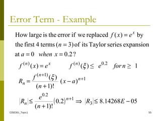
Example 7 – Error Term
)!1(
max
)!1(
)5.0(
2
)!1(
)5.01(
2
)5.0(
)!1(
)(
2)(
3
12
]1,5.0[
1
1
1
121
1
)1(
12)(
+
≤
+
≤
+
−
=
−
+
=
=
+
∈
+
+
+
++
+
+
+
n
e
Error
e
n
Error
n
eError
x
n
f
Error
exf
n
n
n
n
n
n
xkk
ξ
ξ
ξ
ξ