The document discusses correlation as a statistical tool for measuring the relationship between two variables, introducing types of correlation, such as positive, negative, simple, and multiple. It details methods for calculating coefficients of correlation, including Karl Pearson's method, and the use of scatter diagrams to visualize relationships. Additionally, it covers concepts like bivariate distribution and the merits and limitations of various correlation methods.

1. RAI UNIVERSITY, AHMEDABAD 1
Course: MCA
Subject: Computer Oriented Numerical
Statistical Methods
Unit-4
RAI UNIVERSITY, AHMEDABAD

2. RAI UNIVERSITY, AHMEDABAD 2
Unit-IV-Correlation
Sr.
No.
Name of the Topic Page
No.
1 Introduction and Definition of Correlation 2
2 Types of Correlation and examples of correlation 3
3 Coefficient of Correlation, Methods for calculating coefficient of
Correlation.
5
4 Scatter diagram method and its example, Merit and limitations of
Scatter diagram method
6
5 Karl Pearson’s coefficient of correlation and examples based on
its, Properties of Karl Pearson’s coefficient
12
6 Correlation Coefficient for Bivariate Frequency Distribution and
its examples
16
7. Merits and limitations of Karl Pearson’s coefficient 21
8. Probable error and example based on it. 22
9. References 24
10 Exercise 25

3. RAI UNIVERSITY, AHMEDABAD 3
1.1 Introduction:
In this Lesson, we have discussed about the correlation. In which, we have defined
the measure of relationship between two variables...
Suppose we have a set of 30 students in a class and we want to measure the heights
and weights of all the students. We observe that each individual (unit) of the set
assumes two values – one relating to the height and the other to the weight. Such a
distribution in which each individual or unit of the set is made up of two values is
called a bivariate distribution. Some examples of bivariate distribution are
(i) In a class of 60 students the series of marks obtained in two subjects by
all of them.
(ii) The series of sales revenue and advertising expenditure of two companies
in a particular year.
(iii) The series of ages of husbands and wives in a sample of selected married
couples.
Thus in a bivariate distribution, we are given a set of pairs of observations, where
in each pair represents the values of two variables.
The concept of ‘correlation’ is a statistical tool which studies the relationship
between two variables and Correlation Analysis involves various methods and
techniques used for studying and measuring the extent of the relationship between
the two variables.
1.2 Definition:
Two variables are said to be in correlation if the change in one of the variables
results in a change in the other variable.

4. RAI UNIVERSITY, AHMEDABAD 4
2.1 Types of correlation.
Correlation is classified by the following types and they are:
1. Positive and Negative 4. No correlation
2. Simple, Multiple and partial 5. Strong Correlation
3. Linear and non linear. 6. Weak Correlation
1. Positive and Negative
Positive and negative correlation depends on the direction of change of the
Variables. If move variables move in the same direction i.e., when there is an
increase in
The value one variable influenced by an increase in the value of other variable is
called
Positive correlation. If two variables tend to move in opposite directions so that an
Increase in the values of one variable is influenced by decrease in the value of the
other
Variable, then the correlation is said to be negative correlation.
2.Simple and Multiple and Partial:
When we study about only two variables then the correlation is said to be simple

5. RAI UNIVERSITY, AHMEDABAD 5
where as we study about more than two variables is called multiple correlation. In
multiple variable environments, some variables excluded due to some reason
then it is termed as partial correlation
3.Linear and Non-Linear:
The distinction between linear and non-linear correlation is based upon the
consistency of the ratio of change between the variables. If the amount of change
in one variable tends to bear constant ratio to the amount of change in one variable
then the correlation is said to be linear.
Correlation would be called non-linear or curve linear if the amount of change in
one variable does not bear a constant ratio to the amount of change in the other
variable. For example, if we double the amount of rainfall, the production of rice or
wheat, etc., would not necessary be doubled.
4. No Correlation
No correlation occurs when there is no linear dependency between the variables.

6. RAI UNIVERSITY, AHMEDABAD 6
5. Strong Correlation
A correlation is stronger the closer the points are located to one another on the line.
6. Weak Correlation
A correlation is weaker the farther apart the points are located to one another on
the line.
2.2 Some examples of series of positive correlation are:
(i) Heights and weights;
(ii) Household income and expenditure;
(iii) Price and supply of commodities;
(iv) Amount of rainfall and yield of crops.
3.1 Coefficient of Correlation
Correlation is statistical technique used for analyzing the behavior of two
Variables. This analysis refers with the relationship between two or more variables.
Statistical measures of correlation are co-variation between series, not of functional

7. RAI UNIVERSITY, AHMEDABAD 7
Relationship. It is not possible to obtain another variable, if the value of a one
variable Known in one series.
3.2 Methods For calculating Coefficient of Correlation:
4.1 Scatter Diagram Method
Scatter diagram is most popular and easy way of deciding the relation between two
variables. It is a graphical method and ascertain the direction of correlation
between two variables. To construct the scatter diagram take independent variable
on X-Axis and dependent variable on Y Axis. Plot the graph of intersection points
of two variables and decide the relation according to the scatter plot.
1. If all the points fall on a straight line moving from left lower corner to right
upper corner then it is the perfect positive correlation.

8. RAI UNIVERSITY, AHMEDABAD 8
2. If all the points fall on a straight line moving from upper left corner to right
lower corner then it is a perfect negative correlation.
3. If all the points scattered nearby around the line then this will be high or low
degree of positive and negative correlation according to the direction of line.

9. RAI UNIVERSITY, AHMEDABAD 9
4. If all the points scattered every where on the graph and no pattern will be
identified then there is no correlation between the variables.

10. RAI UNIVERSITY, AHMEDABAD 10
4.1.1 Example—Company α decides to use scatter graph method to split its
factory overhead (FOH) into variable and fixed components. Following is the
data which is provided for the analysis.
Mont
h
Units FOH
1 1,520 $36,375
2 1,250 38,000
3 1,750 41,750
4 1,600 42,360
5 2,350 55,080
6 2,100 48,100
7 3,000 59,000
8 2,750 56,800
Solution:

11. RAI UNIVERSITY, AHMEDABAD 11
Fixed Cost = y-intercept = $18,000
Variable Cost per Unit = Slope of Regression Line
To calculate slop we will take two points on line: (0, 18000) and (3500, 68000)
Variable Cost per Unit = (68000 − 18000) ÷ (3500 − 0) = $14.286
4.1.2 Example –Situation: The new commissioner of the American Basketball
League wants to construct a scatter diagram to find out if there is any
relationship between a player’s weight and her height. How should she go
about making her scatter diagram?

12. RAI UNIVERSITY, AHMEDABAD 12
Collect the data (Remember to use 50-100 paired samples).
Draw and label your x and y axes.
Plot the data on the diagram.

13. RAI UNIVERSITY, AHMEDABAD 13
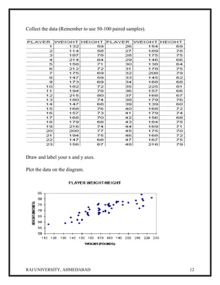
According to this scatter diagram the new commissioner was right. There does
seem to be a positive correlation between a player's weight and her height. In other
words, the taller a player is the more she tends to weight.
4.2 Merits:
(1) This is a simple method of studying correlation between two variables.
(2)More mathematical knowledge is not required in this method.
(3)If one of the pairs of values is extreme, it does not influence much in
deriving the conclusion.
(4)It is the first step in studying the relationship between two variables.
4.3 Limitations:
(1)This method gives an idea about the direction and to some extent the degree
of relationship between the variables, but does not give the exact measure of
the relationship between the variables.
5.1 Karl Pearson’s Coefficient of Correlation
The Karl Pearson’s method is popularly known as Pearson’s Coefficient of
correlation.
One of the most widely used statistics is the coefficient of correlation‘𝑟’ which
measures the degree of association between the two values of related variables
given in the data set. The coefficient of correlation ‘r’ is given by the formula
𝑟 =
∑ 𝑋𝑌
𝑛𝜎𝑥 𝜎 𝑦
=
∑ 𝑋𝑌
√∑ 𝑥2 ∑ 𝑦2
[∵ 𝜎2
𝑥 =
∑ 𝑥2
𝑛
; 𝜎2
𝑦 =
∑ 𝑦2
𝑛
]

14. RAI UNIVERSITY, AHMEDABAD 14
Here 𝑋 = (𝑥 − 𝑥̅); 𝑌 = (𝑦 − 𝑦̅)
𝜎𝑥 =Standard deviation of series 𝑥
𝜎 𝑦 =Standard deviation of series 𝑦
𝑛 = Number of pairs of observations
𝑟 = The (product moment) correction coefficient
This method is to be applied only where deviations of items are taken from actual
mean and not from the assumed mean.
The values of coefficient of correlation ‘𝑟’ obtained from the above formula
always lies between ±1.
When r = +1 it means there is a perfect positive correlation between the variables.
When r = -1 it means there is a perfect negative correlation between the variables.
However if r = 0 there is no relationship between the variables.
5.2 Steps:
1. Find out the mean of the two series 𝑋̅ 𝑎𝑛𝑑 𝑌̅
2. Take deviations of the two series from the respective means 𝑋̅ 𝑎𝑛𝑑 𝑌̅ and
denote x and y.
3. Square the deviations and find the sum of square and denote ∑ 𝑥2
𝑎𝑛𝑑 ∑ 𝑦2
4. Multiply deviations of 𝑋 and 𝑌 i.e., ∑ 𝑋𝑌
5. Substitute the values of ∑ 𝑋𝑌, ∑ 𝑥2
𝑎𝑛𝑑 ∑ 𝑦2
in the formula.
5.3 Properties of correlation Co-efficient:
(1) The correlation coefficient lies between -1 and +1.
(2)The correlation co-efficient is independent of change of origin and scale.
(3)The correlation co-efficient is an absolute number and it is independent of
units of measurement.

15. RAI UNIVERSITY, AHMEDABAD 15
(4) 𝑟2
always lies between 0 and 1 i.e. 0 ≤ 𝑟2
≤ 1
5.1.1 Example:- Making use of the data summarized below, calculate the
coefficient of correlation
X 3 5 7 3 2
Y 2 4 6 2 1
Solution:
First of All 𝑋̅ =
∑ 𝑥 𝑖
𝑛
and 𝑌̅ =
∑ 𝑦 𝑖
𝑛
∴ 𝑋̅ =
20
5
= 4 and 𝑌̅ =
15
5
= 3
𝒙 𝒚 𝑿 = (𝒙 − 𝑿)̅̅̅̅ 𝒀 = (𝒚 − 𝒀̅) 𝒙𝒚 𝒙 𝟐
𝒚 𝟐
3 2 -1 -1 1 1 1
5 4 1 1 1 1 1
7 6 3 3 9 9 9
3 2 -1 -1 1 1 1
2 1 -2 -2 4 4 4
16 16 16
𝑟 =
∑ 𝑋𝑌
√∑ 𝑥2 ∑ 𝑦2
𝑟 =
16
√16×16
𝑟 =
16
16
𝑟 = 1
5.1.2Example:- Making use of the data summarized below, calculate the
coefficient of correlation .

16. RAI UNIVERSITY, AHMEDABAD 16
Case A B C D E F G H
X 10 9 6 10 12 13 11 9
Y 9 4 6 9 11 13 8 4
Solution:-
First of all we find
𝑥̅ =
∑𝑥
𝑛
=
80
8
= 10 , 𝑦̅ =
∑𝑦
𝑛
=
64
8
= 8
Case 𝒙 𝒙 − 𝟏𝟎 = 𝑿 𝑿 𝟐 𝒚 𝒚 − 𝟖 = 𝒀 𝒀 𝟐 𝑿𝒀
A 10 0 0 9 1 1 0
B 9 -4 16 4 -4 16 16
C 6 -1 1 6 -2 4 2
D 10 0 0 9 +1 1 0
E 12 +2 4 11 +3 9 6
F 13 +3 9 13 +5 25 15
G 11 +1 1 8 0 0 0
H 9 -1 1 4 -4 16 4
𝒏
= 𝟖
∑𝑥
= 80
∑𝑋 = 0 ∑𝑋2
= 32
∑𝑦
= 64
∑𝑌 = 0 ∑𝑌2
= 72
∑𝑋𝑌
= 43

17. RAI UNIVERSITY, AHMEDABAD 17
𝑟 =
∑ 𝑋𝑌
√∑ 𝑋2 ∑ 𝑌2
𝑟 =
43
√32 × 72
𝑟 =
43
√2304
𝑟 =
43
48
= +0.896
6.1 Correlation Coefficient for Bivariate frequency Distribution:
When the number of observations is too large, the data are usually classified in to a
two-way table known as a bivariate table. A bivariate frequency table is given
below.
0-10 10-20 20-30 30-40 40-50 𝒇 𝒚
0-10 1 3 5 2 1 12
10-20 2 4 6 8 2 22
20-30 3 0 7 9 4 23
30-40 4 7 10 7 20 48
40-50 1 2 5 3 4 15
𝒇 𝒙 11 16 33 29 31 120
In the above table a bivariate frequency distribution of marks of mathematics and
marks of science of 120 students are shown. The marks of mathematics are
denoted by 𝑥 and the marks of science are denoted by 𝑦.Both the variables 𝑥 and 𝑦
are classified into groups 0-10,10-20,…etc. The marks in science of different
groups are represented in rows. In the first cell the frequency is 1, which indicates
that there is 1student getting marks between 0-10 in science. The frequency of the
cell of first row and second column is 3 which means there are 3 students getting
𝑥
𝑦

18. RAI UNIVERSITY, AHMEDABAD 18
marks in mathematics between 10-20 and in science between 0-10.The different
values of 𝑓𝑦 show the total number of students securing marks in science in the
corresponding groups. Similarly the different values of 𝑓𝑥 show the total number of
students securing marks in mathematics in the corresponding groups.It is obvious
that ∑ 𝑓𝑥 = ∑ 𝑓𝑦 = 𝑛 (Total Frequency)
The following formula is used for calculating correlation co-efficient for the data
given in bivariate table.
𝑟 =
𝑛 ∑ 𝑓𝑢𝑣 − ∑ 𝑢𝑓𝑢. ∑ 𝑣𝑓𝑣
√𝑛 ∑ 𝑢2 𝑓𝑢 − (∑ 𝑢𝑓𝑢)2 × √𝑛 ∑ 𝑣2 𝑓𝑣 − (∑ 𝑣𝑓𝑣)2
The required values in the above formula can be obtained as follows.
(i) Denote one variable by 𝑋 and another variable by 𝑌.
(ii) Denote mid-value of 𝑋 by 𝑥 and mid-value 𝑌 by 𝑦.
(iii) Obtain 𝑢 and 𝑣 by the formula
𝑢 =
𝑥−𝐴
𝐶 𝑥
𝑣 =
𝑦−𝐵
𝐶 𝑦
Where 𝐴 and 𝐵 are assumed means of 𝑋 and 𝑌 respectively and 𝐶 𝑥 and 𝐶 𝑦 are the
class intervals of variables 𝑥 and 𝑦. It should be noted that frequency of 𝑥 and
frequency of 𝑣 will be the same as frequency of 𝑦. Hence 𝑓𝑥 will be 𝑓𝑢 and 𝑓𝑦 will
be 𝑓𝑣.
(iv) For each class of 𝑥 multiply 𝑢 and 𝑓𝑢 and obtain ∑ 𝑢𝑓𝑢 similarly obtain
∑ 𝑣𝑓𝑣.
(v) For each group of 𝑥 multiply 𝑢𝑓𝑢 by 𝑢 and obtain ∑ 𝑢2
𝑓𝑢. Similarly
obtain ∑ 𝑣2
𝑓𝑣.
(vi) For each cell find the produced of 𝑓, 𝑢 𝑎𝑛𝑑 𝑣 and obtain 𝑓𝑢𝑣 for each
cell. From them find ∑ 𝑓𝑢𝑣.
The value of 𝑟 can be obtained by substituting these values in the formula.
6.1.1 Example—

19. RAI UNIVERSITY, AHMEDABAD 19
Find the coefficient of correlation from the following data:
Age of Wife
Solution: We Know that
𝑟 =
𝑛 ∑ 𝑓𝑢𝑣 − ∑ 𝑢𝑓𝑢. ∑ 𝑣𝑓𝑣
√𝑛 ∑ 𝑢2 𝑓𝑢 − (∑ 𝑢𝑓𝑢)2 × √𝑛 ∑ 𝑣2 𝑓𝑣 − (∑ 𝑣𝑓𝑣)2
Here 𝑛 = ∑ 𝑓𝑥 = ∑ 𝑓𝑦 = 140
𝑢 =
𝑥−25
10
and 𝑣 =
𝑦−25
10
All the values required in the formula can be available from the table. We have to
obtain the values of 𝑓𝑢𝑣 for each cell. For the first cell 𝑓 = 20, 𝑢 = −1 and 𝑣 =
−1. Hence the value of 𝑓𝑢𝑣 for the first cell is 20(-1)(-1)=20. Similarly for the last
cell the values of 𝑓, 𝑢 𝑎𝑛𝑑 𝑣 are respectively 6,2 and 2.
Therefore, 𝑓𝑢𝑣 = 6(2)(2) = 24.
Thus the values of 𝑓𝑢𝑣 for each cell can be obtained. These values are shown in
brackets in each cell.
Age
Of
Husbands
10-20 20-30 30-40 40-50
10-20 20 26 - -
20-30 8 14 37 -
30-40 - 4 18 3
40-50 - - 4 6

20. RAI UNIVERSITY, AHMEDABAD 20
↓ → 𝒙
y
10-20 20-30 30-40 40-50 𝒇 𝒚 M.V.
𝒚
𝒗 𝒗𝒇 𝒗 𝒗 𝟐
𝒇 𝒗 𝒇𝒖𝒗
10-20 (20)
20
(0)
26
46 15 -1 -46 46 20
20-30 (0)
8
(0)
14
(0)
37
59 25 0 0 0 0
30-40 (0)
4
(18)
18
(6)
3
25 35 1 25 25 24
40-50 (8)
4
(24)
6
10 45 2 20 40 32
𝒇 𝒙 28 44 59 9 140 -1 111 76
M.V. 𝒙 15 25 35 45
𝒖 -1 0 1 22
𝒖𝒇 𝒖 -28 0 59 18 49
𝒖 𝟐
𝒇 𝒖 28 0 59 36 123
𝒇𝒖𝒗 20 0 26 30 76
Row- wise and column –wise totals of these values are shown in the last row and
the last column respectively .From them ∑ 𝑓𝑢𝑣 is obtained .The values of ∑ 𝑓𝑢𝑣
obtained from rows and columns should be equal. In the given example
∑ 𝑓𝑢𝑣 = 76.
Now putting these values in the formula, we get
𝑟 =
140(76)−(49)(−1)
√140(123)−(49)2×√140(111)−(−1)2
𝑟 =
10689
√14819×√15539
𝑟 = 0.70

21. RAI UNIVERSITY, AHMEDABAD 21
6.1.2 Example—
Find correlation coefficient from the following data:
Scores 18 19 20 21 22
200-250 3 3 2 1 -
250-300 - 2 4 2 2
300-350 3 5 5 2 -
350-400 - 1 2 3 3
400-450 - - 2 4 1
Solution:
↓ → 𝒙
y
18 19 20 21 22 𝒇 𝒚 M.V.
𝒚
𝒗 𝒗𝒇 𝒗 𝒗 𝟐
𝒇 𝒗 𝒇𝒖𝒗
200-250 (12)
3
(6)
3
(0)
2
(-2)
1 9 225 -2 -18 36 16
250-300 (2)
2
(0)
4
(-2)
2
(-4)
2 10 275 -1 -10 10 -4
300-350 (0)
3
(0)
5
(0)
5 15 325 0 0 0 0
350-400 (-1)
1
(0)
2
(3)
3
(6)
3 9 375 1 9 9 8
400-450 (0)
2
(8)
4
(4)
1 7 425 2 14 28 12
𝒇 𝒙 6 11 15 12 6 50 -5 83 32
M.V. 𝒙 18 19 20 21 22
𝒖 -2 -1 0 1 2

22. RAI UNIVERSITY, AHMEDABAD 22
𝒖𝒇 𝒖 -12 -11 0 12 12 1
𝒖 𝟐
𝒇 𝒖 24 11 0 12 24 71
𝒇𝒖𝒗 12 7 0 7 6 32
We shall denote age by 𝑦 and ages 18,19…shall be taken as mid values.
𝑟 =
𝑛 ∑ 𝑓𝑢𝑣−∑ 𝑢𝑓𝑢.∑ 𝑣𝑓𝑣
√𝑛 ∑ 𝑢2 𝑓𝑢−(∑ 𝑢𝑓𝑢)2×√𝑛 ∑ 𝑣2 𝑓𝑣−(∑ 𝑣𝑓𝑣)2
𝑟 =
50(32)−(1)(−5)
√50(71)−(1)2×√50(83)−(−5)2
𝑟 =
1605
√3549×√4125
𝑟 = 0.42
7.1 Merits of Karl Pearson’s correlation coefficient:
1. Karl Pearson’s co-efficient of correlation is the best measure for
representing the relationship between two variables.
2. The degree and direction of the relationship between the variables can be
obtained by it.
7.2 Limitations of Karl Pearson’s correlation coefficient:
1. It is based on the assumption of linearity of relationship between the
variables.
2. The computation by this method is difficult compared to other methods
3. The correlation co-efficient is highly influenced by extreme pairs of
observations.
4. It is always difficult to interprete the correlation co-efficient, correctly.

23. RAI UNIVERSITY, AHMEDABAD 23
8.1 Probable Error:
Generally we obtain correlation co-efficient of a sample drawn from a bivariate
population. If different samples of the same size are drawn from a given
population, we get different values of 𝑟. All these values of 𝑟 differ from the
actual value of the population correlation co-efficient. The average of the absolute
differences of correlation Co-efficients obtained from all possible samples and the
population correlation co-efficient is known as probable error of the correlation
Co-efficient.
The value of probable error depends upon the size of the sample. If the sample is
large, the value of probable error is small. From the value of the sample correlation
co-efficient we can estimate the population correlation co-efficient, and with the
help of probable error we can determine whether the correlation in the population
is significant or not.
If a sample of size 𝑛 is drawn from a bivariate population and if 𝑟 is its correlation
co-efficient ,then the probable error (P.E) can be found out by the following
formula:
𝑃. 𝐸. =
0.6745(1 − 𝑟2
)
√ 𝑛
The following rules can be applied to judge whether the correlation in the
population is significant or not:
(1)If 𝑟 < 𝑃. 𝐸., there is no evidence of correlation in the population.
i.e. the correlation in the population is not significant.
(2)If 𝑟 > 6(𝑃. 𝐸. ), there is evidence of significant correlation in the population.
Moreover with the help of probable error we can determine the limits. Within
which the population correlation co-efficient is expected to lie.
The probable limits of the population correlation co-efficient are 𝑟 ± 𝑃. 𝐸.
8.1.1 Example—

24. RAI UNIVERSITY, AHMEDABAD 24
The correlation co-efficient obtained from 𝒂 sample of 16 pairs of
observations drawn from a population is 0.7,calculate the probable error of
the correlation co-efficient and interprete it. Also find the limits of the
population correlation co-efficient.
Solution:
Here 𝑛 = 16 and 𝑟 = 0.7
∴ Probable error =
0.6745(1−𝑟2)
√ 𝑛
∴ Probable error =
0.6745(1−(0.7)2)
√16
∴ Probable error = 0.086
Here 𝑟 = 0.7 𝑎𝑛𝑑 6(𝑃. 𝐸) =6 (0.086) = 0.516 i.e. 𝑟 > 6(𝑃. 𝐸. )
Thus there is significant correlation between the variables.
The probable limit of the population co-efficient is
𝑟 ± 𝑃. 𝐸. = 0.7 ± 0.086 = 0.614 𝑡𝑜 0.786
This means that the population correlation co-efficient will most probably lie
between 0.614 and 0.786.

25. RAI UNIVERSITY, AHMEDABAD 25
References and website Name:
1. Statistical Methods by S.P.Gupta
2. Business Statistics (B.S. Shah Prakashan)
3. http://www.tutorhelpdesk.com/homeworkhelp/Statistics-/Scatter-Diagram-
Method-Assignment-Help.html
4. http://shakehandwithlife.blogspot.in/2014/09/measures-of-correlation.html
5. http://www.spcforexcel.com/files/images/positivecorrelation.png
6. http://www.spcforexcel.com/files/images/negativecorrelation.png
7. http://www.dhsbpsychology.co.uk/wp-
content/uploads/2013/04/Correlations.jpg

26. RAI UNIVERSITY, AHMEDABAD 26
EXERCISE
Q-1 Evaluate the following Questions:
1. Find Pearson’s correlation co-efficient.
Wage 100 101 102 102 100 99 97 98 96 95
Cost of
living Index
98 99 99 97 95 92 95 94 90 91
2. Find correlation Coefficient.
x 300 350 400 450 500 550 600 650 700
y 800 900 1000 1100 1200 1300 1400 1500 1600
3. Find correlation co-efficient from the following data:
Scores 18 19 20 21 22
200-250 3 3 2 1 -
250-300 - 2 4 2 2
300-350 3 5 5 2 -
350-400 - 1 2 3 3
400-450 - - 2 4 1
4. The Correlation co-efficient for a sample drawn form a bivariate population
is 0.6 and its probable error is 0.05396.Find number of pairs of the sample.
Also find the probable limits for the population correlation co-efficient.
5. Find number of pairs from the following data:
𝑟 = 0.5; ∑ 𝑥𝑦 =120;∑ 𝑥2
= 90; 𝑆 𝑦 = 8.