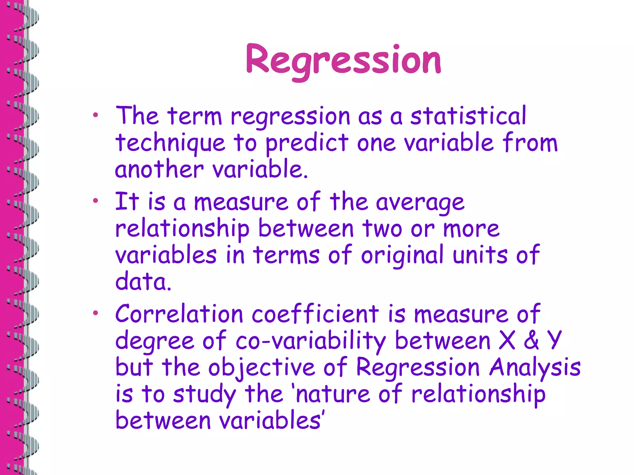
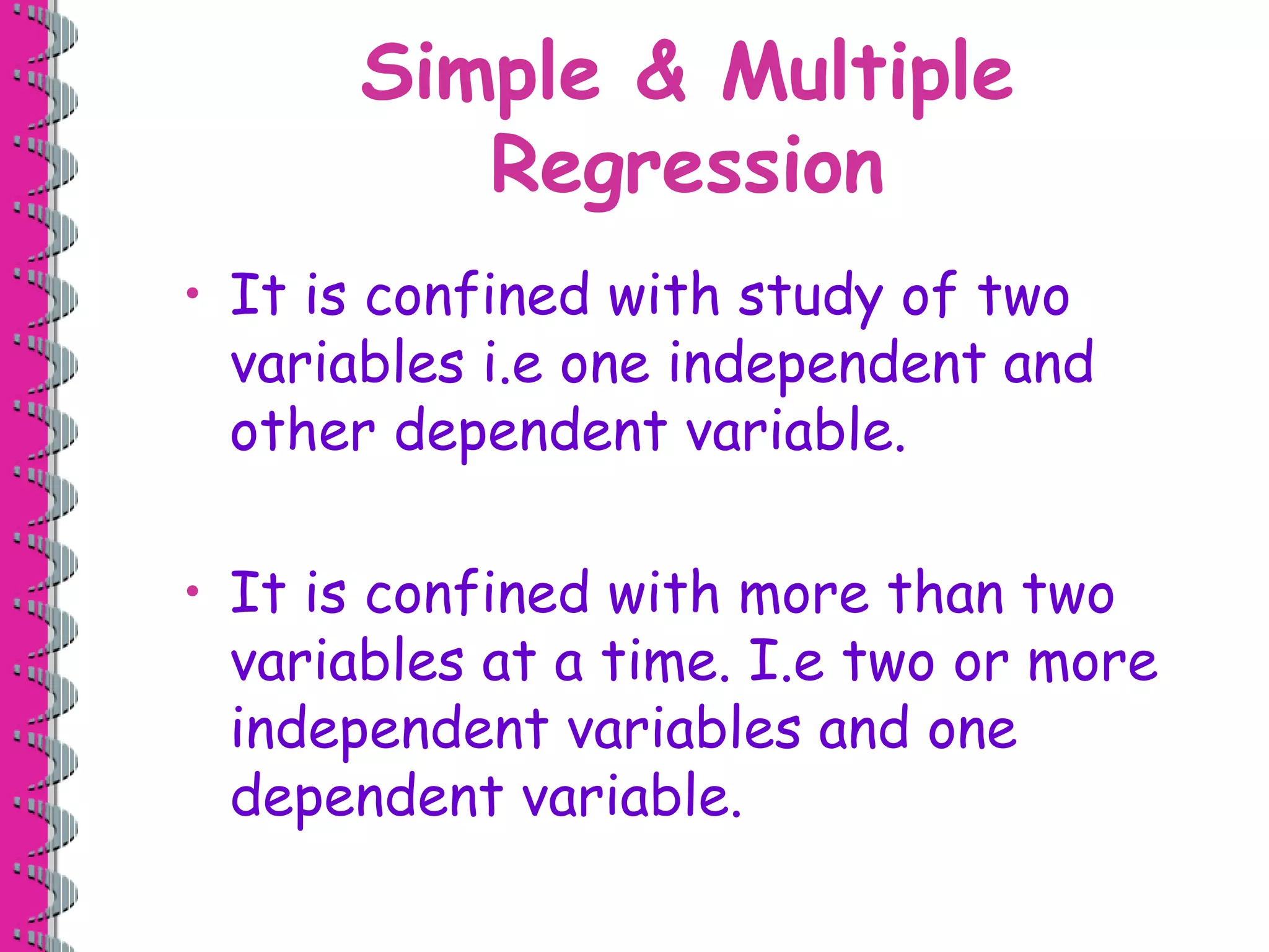
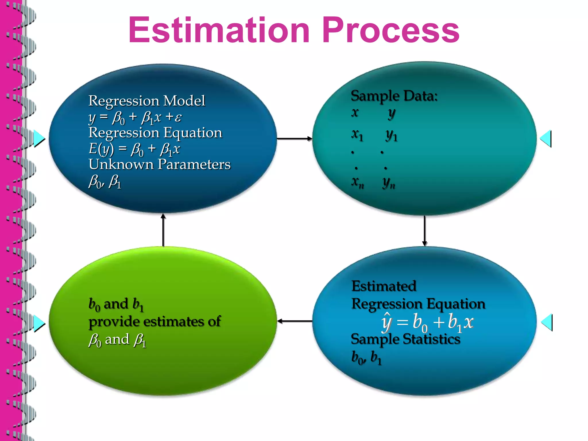
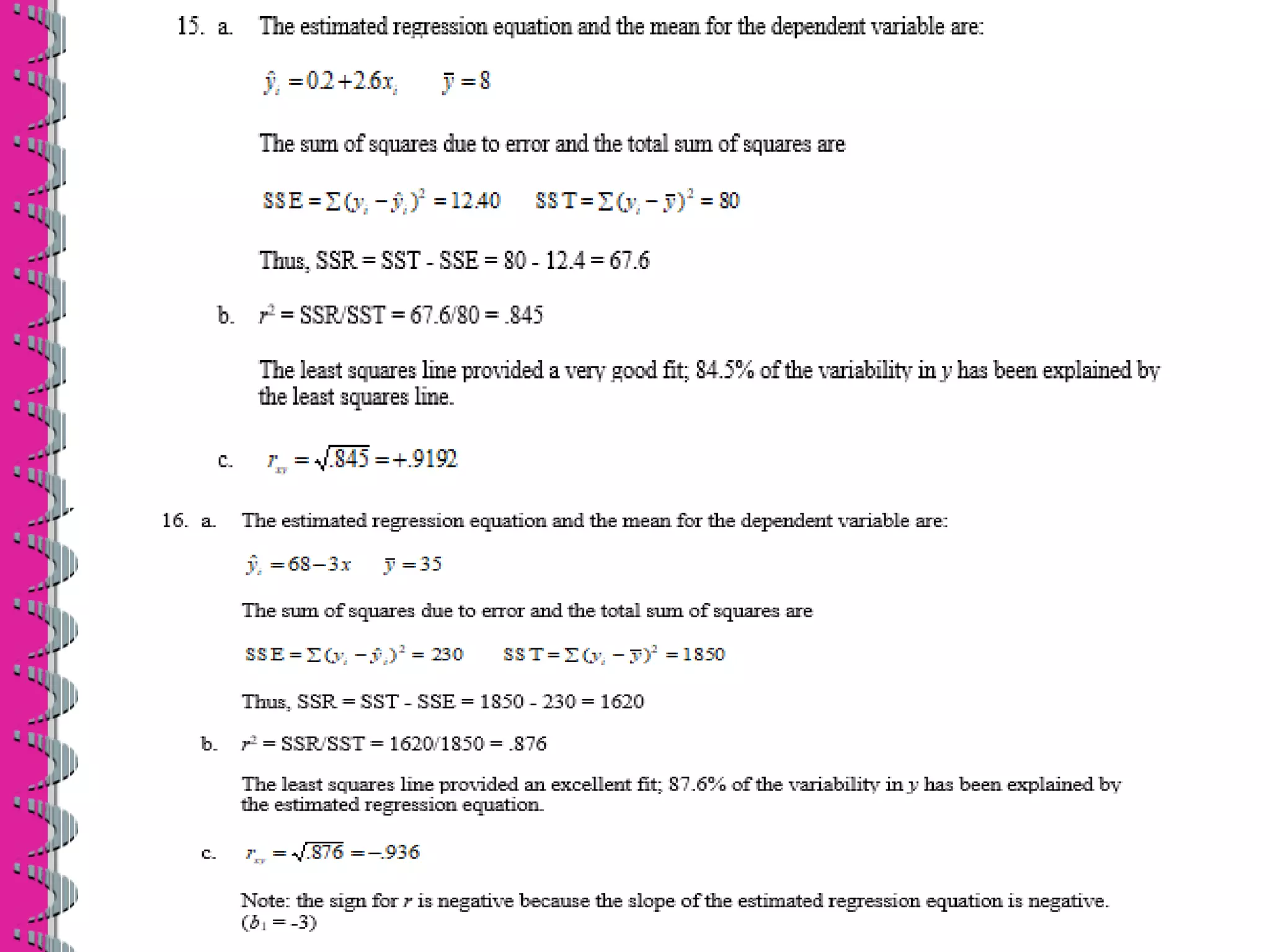
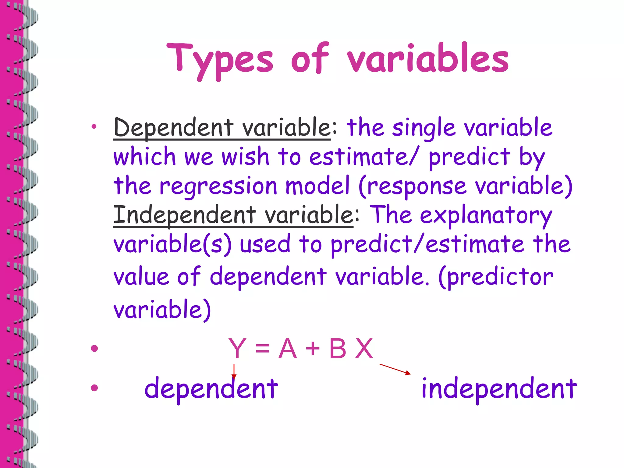
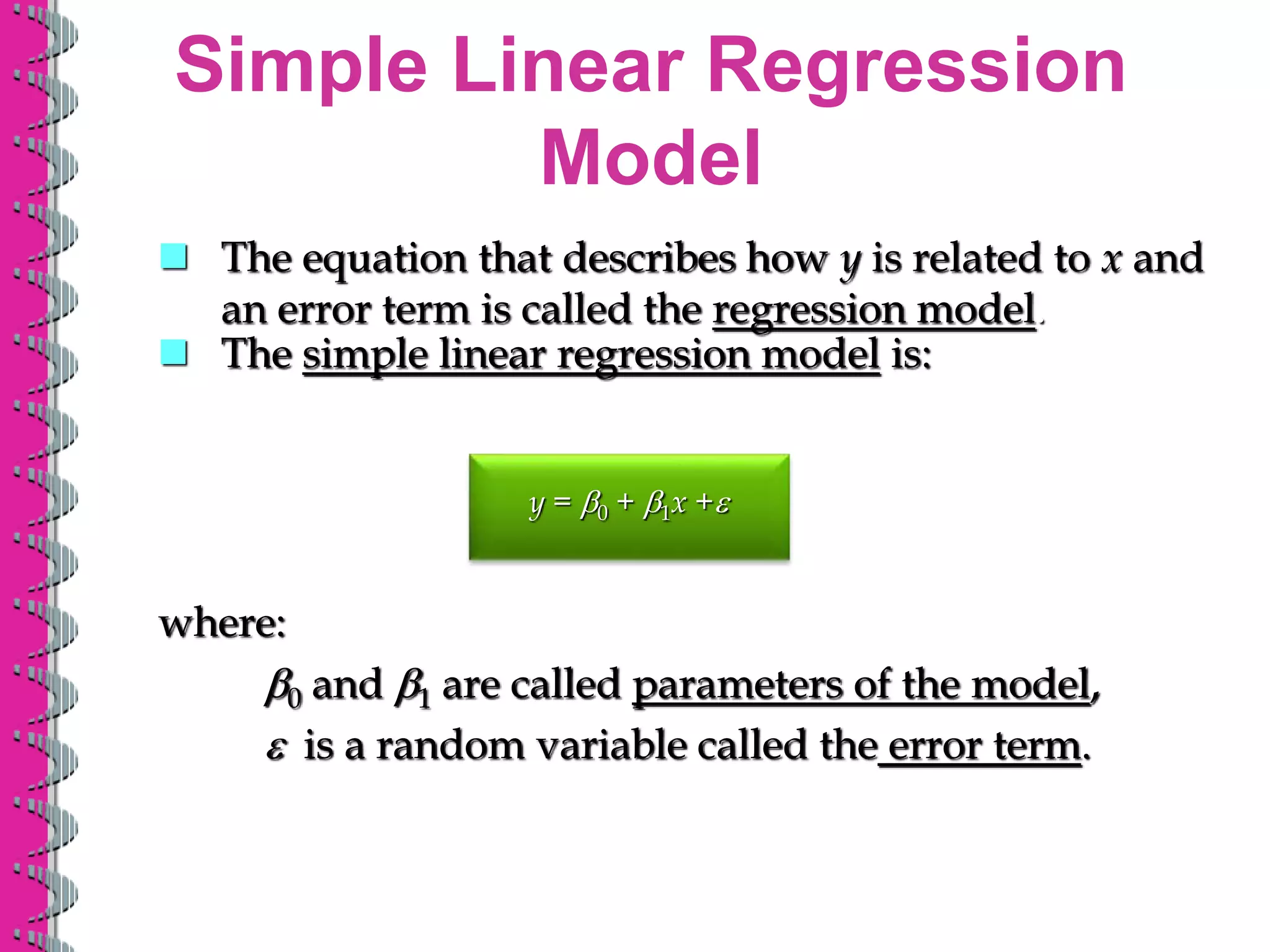
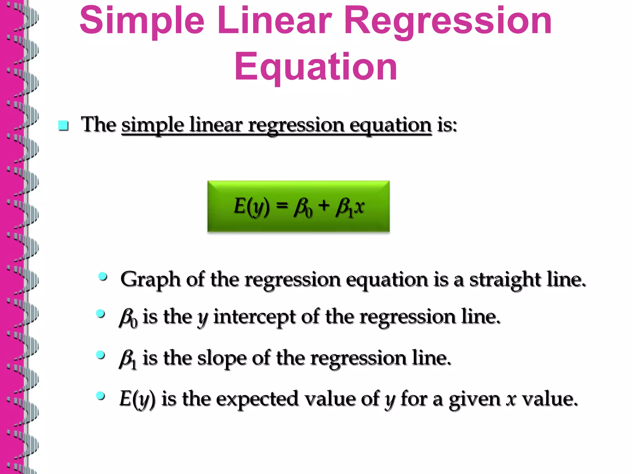
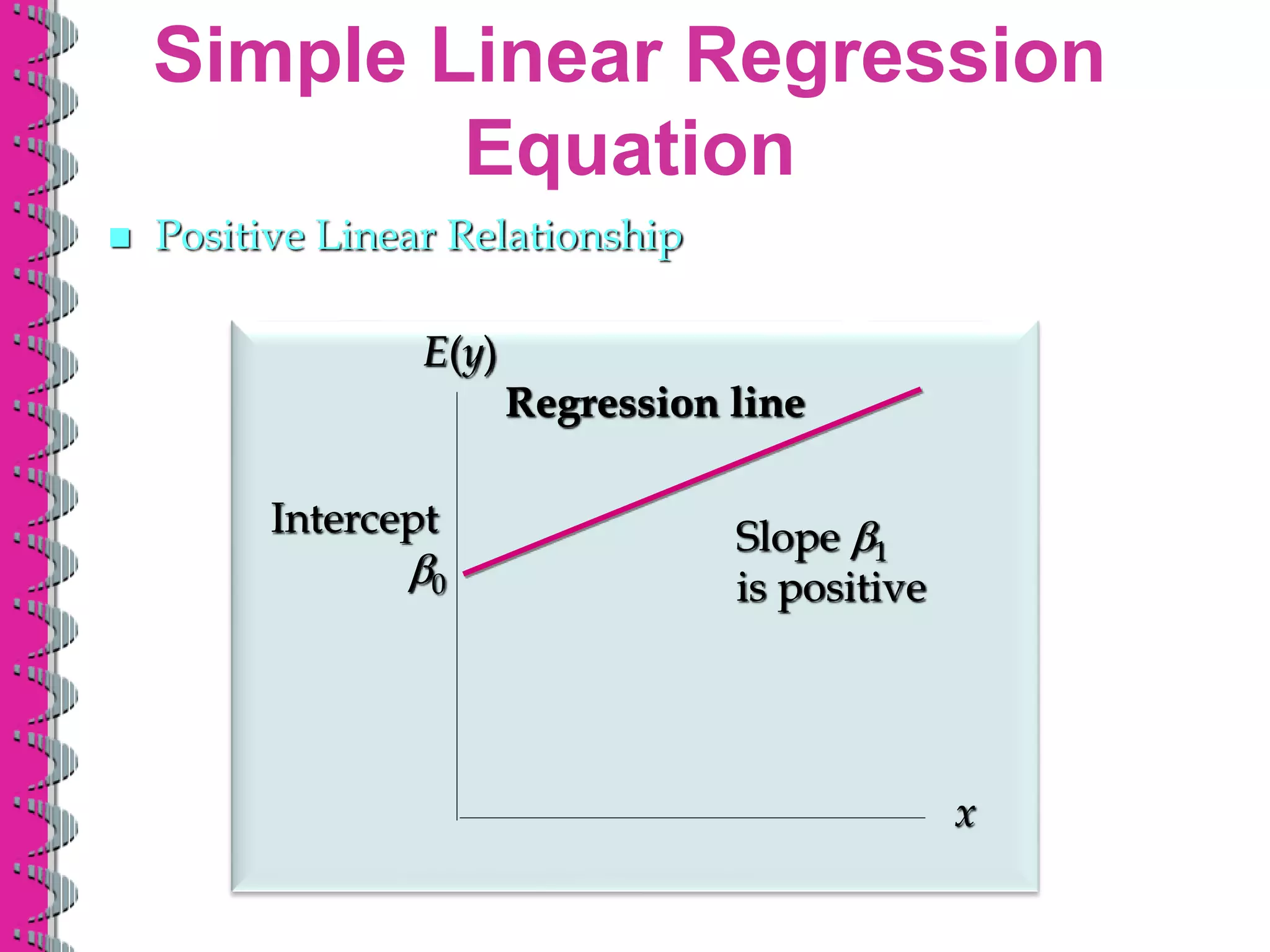
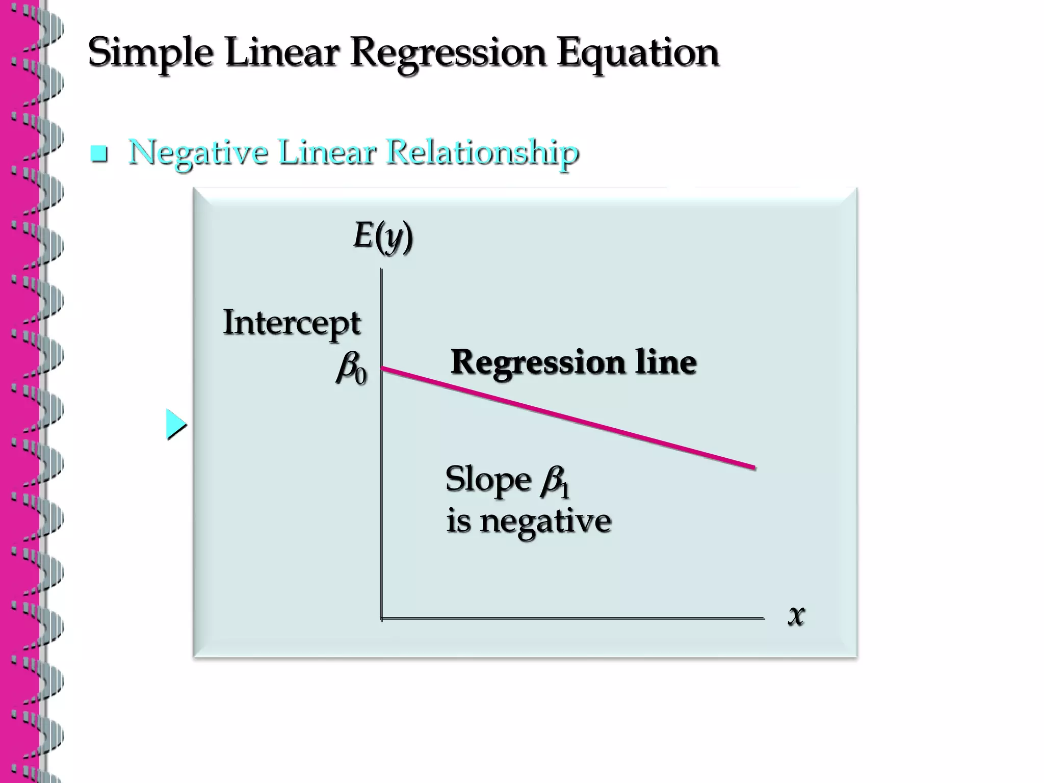
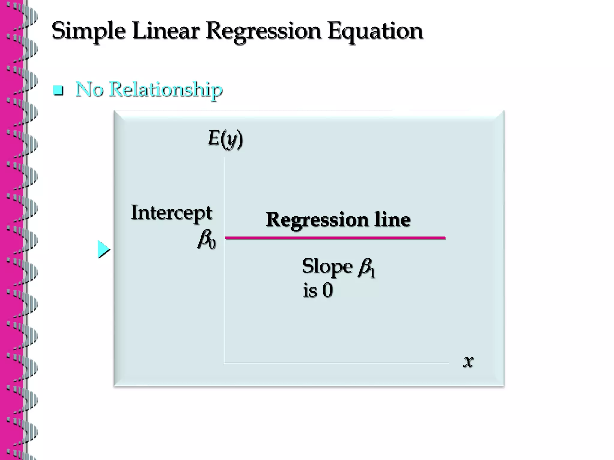
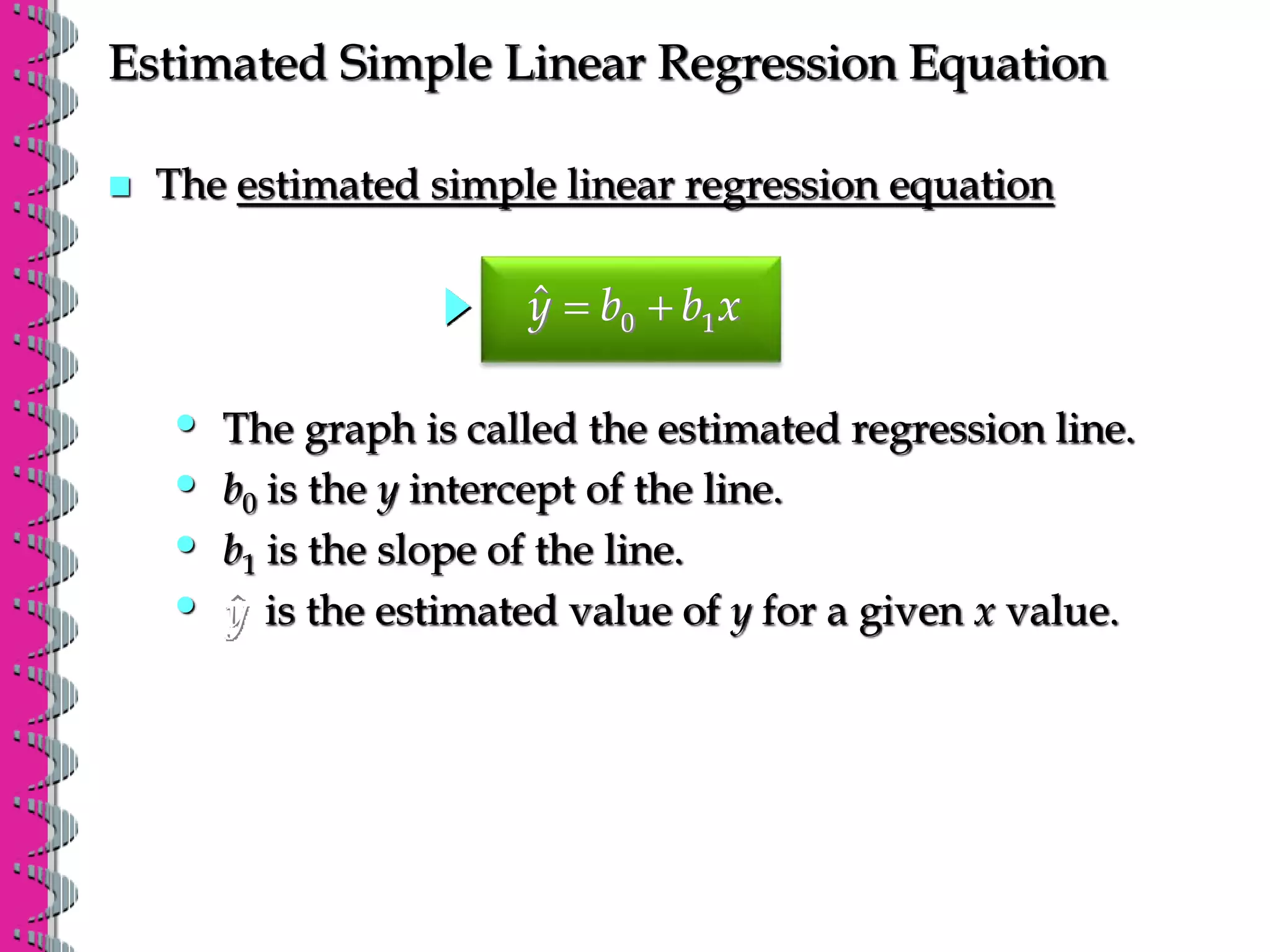
- Regression analysis is used to study the relationship between variables and predict how the value of one variable changes with the other. It is one of the most commonly used tools for business analysis. - Simple linear regression analyzes the relationship between one independent variable and one dependent variable. The regression equation estimates the dependent variable as a linear function of the independent variable. 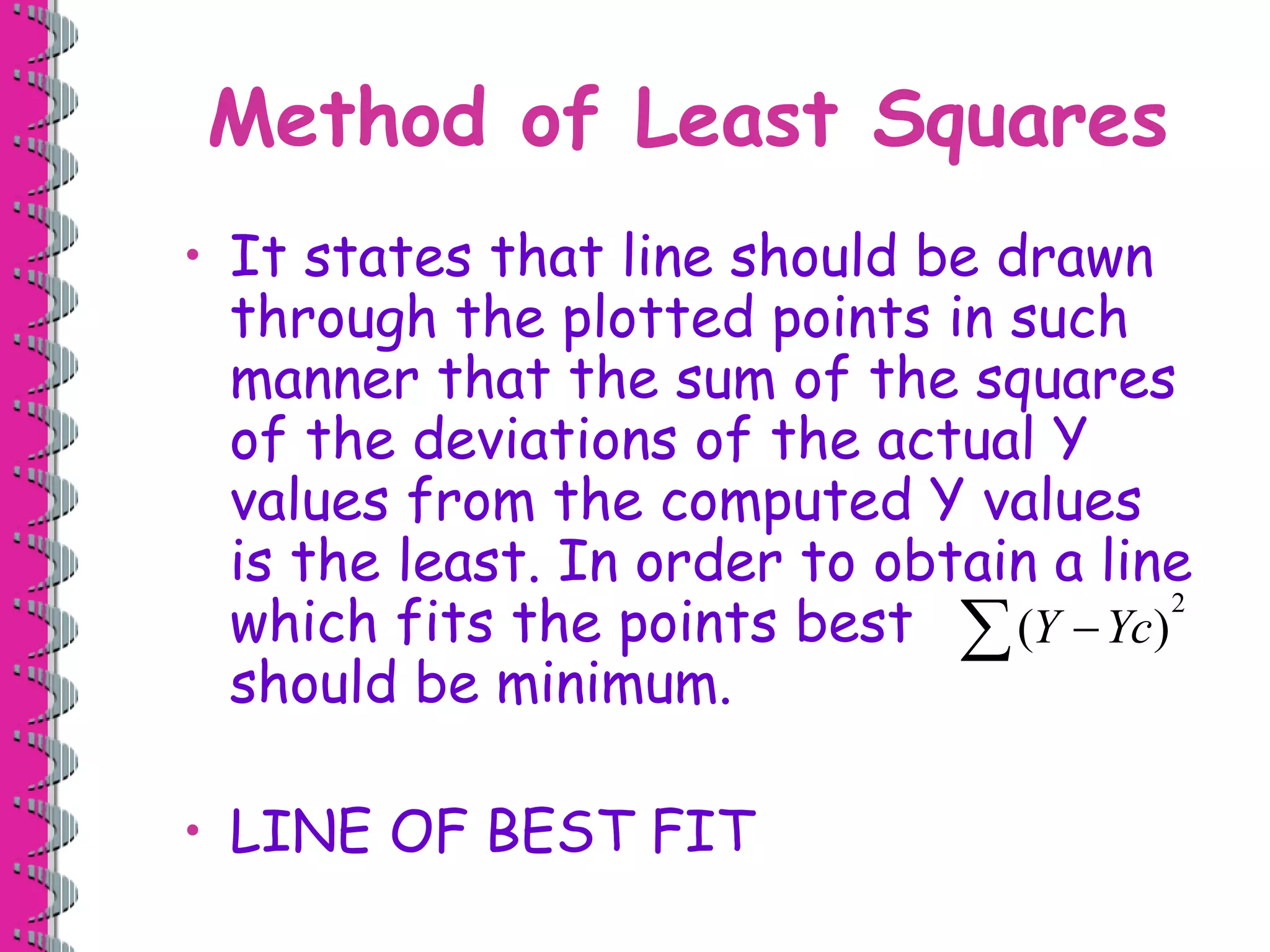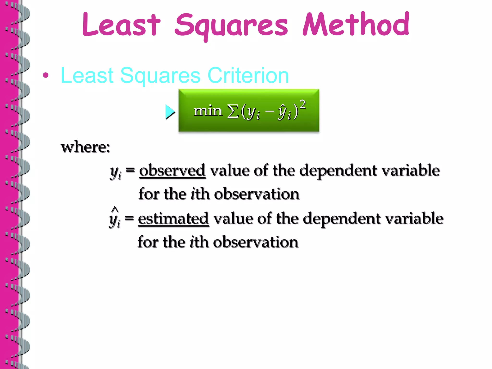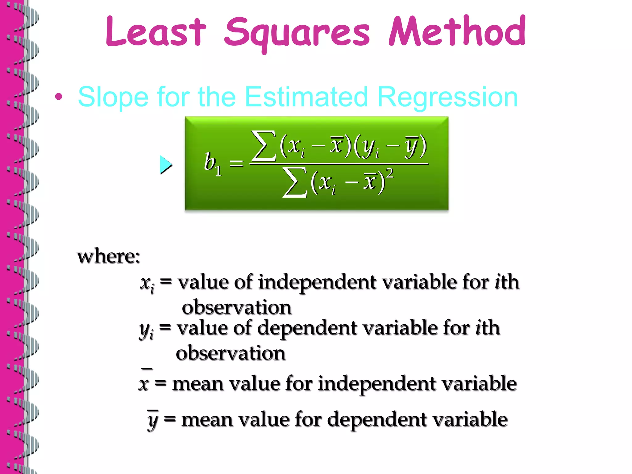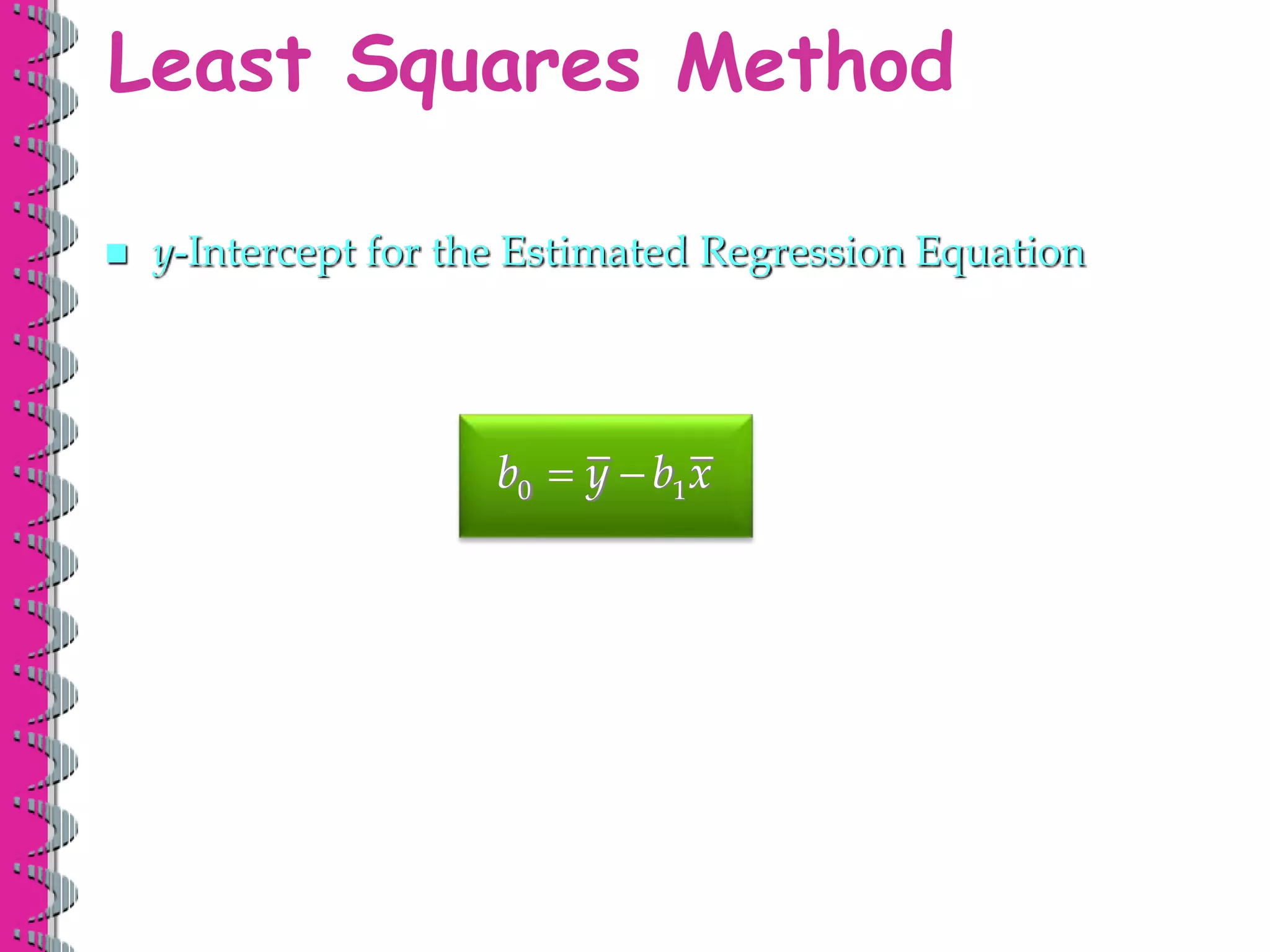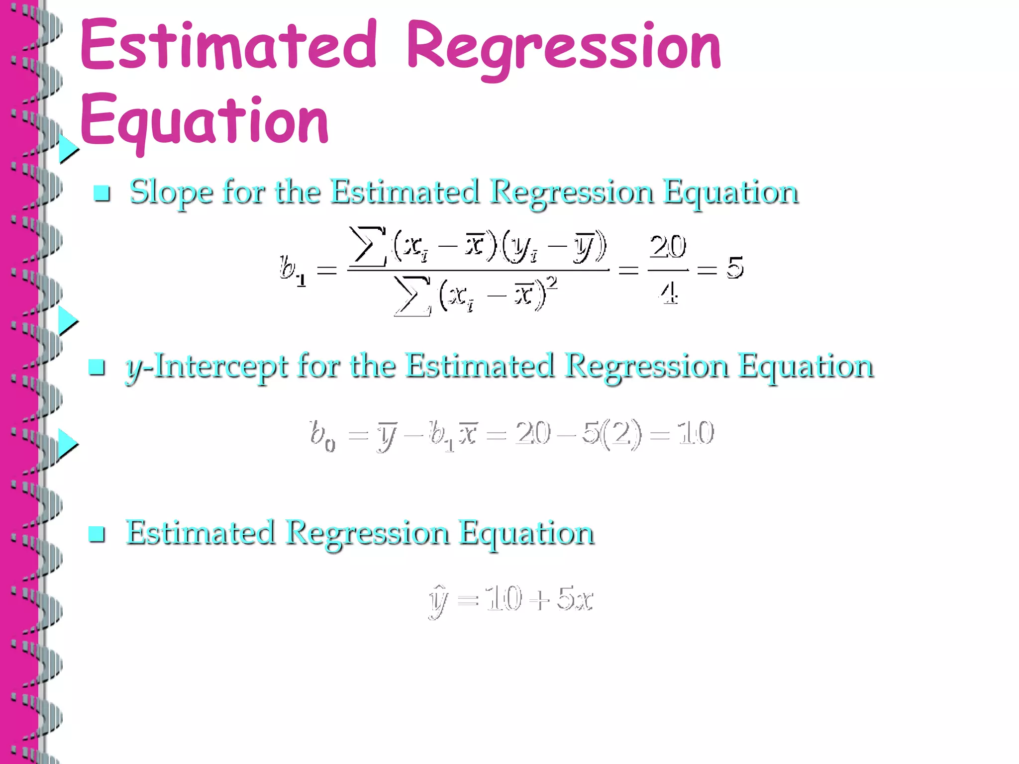- Least squares regression fits a line to the data by minimizing the sum of the squared residuals, providing estimates of the slope and y-intercept coefficients in the regression equation.

1. Regression
Analysis…

2. Regression Analysis: the study of the
relationship between variables
Regression Analysis: one of the most
commonly used tools for business analysis
Easy to use and applies to many situations
Regression Analysis

3. Regression
• The term regression as a statistical
technique to predict one variable from
another variable.
• It is a measure of the average
relationship between two or more
variables in terms of original units of
data.
• Correlation coefficient is measure of
degree of co-variability between X & Y
but the objective of Regression Analysis
is to study the ‘nature of relationship
between variables’

4. Types of Regression
• Linear and Non Linear Regression-
• If the given points are plotted on a
graph paper , the points so obtained on
the scatter diagram will more/less
concentrated round a curve called the
curve of Regression.
• If the regression curve is a straight line
then linear otherwise non linear/curved
regression.

5. Simple & Multiple
Regression
• It is confined with study of two
variables i.e one independent and
other dependent variable.
• It is confined with more than two
variables at a time. I.e two or more
independent variables and one
dependent variable.

6. Types of variables
• Dependent variable: the single variable
which we wish to estimate/ predict by
the regression model (response variable)
Independent variable: The explanatory
variable(s) used to predict/estimate the
value of dependent variable. (predictor
variable)
• Y = A + B X
• dependent independent

7. Simple Linear Regression
Model
y = b0 + b1x +e
where:
b0 and b1 are called parameters of the model,
e is a random variable called the error term.
 The simple linear regression model is:
 The equation that describes how y is related to x and
an error term is called the regression model.

8. Simple Linear Regression
Equation
 The simple linear regression equation is:
• E(y) is the expected value of y for a given x value.
• b1 is the slope of the regression line.
• b0 is the y intercept of the regression line.
• Graph of the regression equation is a straight line.
E(y) = b0 + b1x

9. Simple Linear Regression
Equation
 Positive Linear Relationship
E(y)
x
Slope b1
is positive
Regression line
Intercept
b0

10. Simple Linear Regression Equation
 Negative Linear Relationship
E(y)
x
Slope b1
is negative
Regression line
Intercept
b0

11. Simple Linear Regression Equation
 No Relationship
E(y)
x
Slope b1
is 0
Regression line
Intercept
b0

12. Estimated Simple Linear Regression Equation
 The estimated simple linear regression equation
0 1
ŷ b b x
 
• is the estimated value of y for a given x value.
ŷ
• b1 is the slope of the line.
• b0 is the y intercept of the line.
• The graph is called the estimated regression line.

13. Estimation Process
Regression Model
y = b0 + b1x +e
Regression Equation
E(y) = b0 + b1x
Unknown Parameters
b0, b1
Sample Data:
x y
x1 y1
. .
. .
xn yn
b0 and b1
provide estimates of
b0 and b1
Estimated
Regression Equation
Sample Statistics
b0, b1
0 1
ŷ b b x
 

14. Method of Least Squares
• It states that line should be drawn
through the plotted points in such
manner that the sum of the squares
of the deviations of the actual Y
values from the computed Y values
is the least. In order to obtain a line
which fits the points best
should be minimum.
• LINE OF BEST FIT
2
( )
Y Yc



15. Least Squares Method
• Least Squares Criterion
min (y y
i i

  )2
where:
yi = observed value of the dependent variable
for the ith observation
^
yi = estimated value of the dependent variable
for the ith observation

16. • Slope for the Estimated Regression
1 2
( )( )
( )
i i
i
x x y y
b
x x
 




Least Squares Method
where:
xi = value of independent variable for ith
observation
_
y = mean value for dependent variable
_
x = mean value for independent variable
yi = value of dependent variable for ith
observation

17.  y-Intercept for the Estimated Regression Equation
Least Squares Method
0 1
b y b x
 

18. Reed Auto periodically has a special
week-long sale.
As part of the advertising campaign Reed
runs one or
more television commercials during the
weekend
preceding the sale. Data from a sample
of 5 previous
sales are shown on the next slide.
Simple Linear Regression
 Example: Reed Auto Sales

19. Simple Linear Regression
 Example: Reed Auto Sales
Number of
TV Ads (x)
Number of
Cars Sold (y)
1
3
2
1
3
14
24
18
17
27
Sx = 10 Sy = 100
2
x  20
y 

20. Estimated Regression
Equation
ˆ 10 5
y x
 
1 2
( )( ) 20
5
( ) 4
i i
i
x x y y
b
x x
 
  



0 1 20 5(2) 10
b y b x
    
 Slope for the Estimated Regression Equation
 y-Intercept for the Estimated Regression Equation
 Estimated Regression Equation

21. Practice Example

25. Practice HW
• Pg no. 609, q1
• Pg no. 610 q3, q5
• Pg no. 612 q7

26. Coefficient of Determination
• Relationship Among SST, SSR, SSE
where:
SST = total sum of squares
SSR = sum of squares due to regression
SSE = sum of squares due to error
SST = SSR + SSE
2
( )
i
y y

 2
ˆ
( )
i
y y
 
 2
ˆ
( )
i i
y y
 


28.  The coefficient of determination is:
Coefficient of Determination
where:
SSR = sum of squares due to regression
SST = total sum of squares
r2 = SSR/SST

29. Coefficient of Determination
r2 = SSR/SST = 100/114 = .8772
The regression relationship is very strong; 87.72%
of the variability in the number of cars sold can be
explained by the linear relationship between the
number of TV ads and the number of cars sold.

30. Sample Correlation Coefficient
2
1)
of
(sign r
b
rxy 
ion
Determinat
of
t
Coefficien
)
of
(sign 1
b
rxy 
where:
b1 = the slope of the estimated regression
equation x
b
b
y 1
0
ˆ 


31. 2
1)
of
(sign r
b
rxy 
The sign of b1 in the equation is “+”.
ˆ 10 5
y x
 
= + .8772
xy
r
Sample Correlation Coefficient
rxy = +.9366