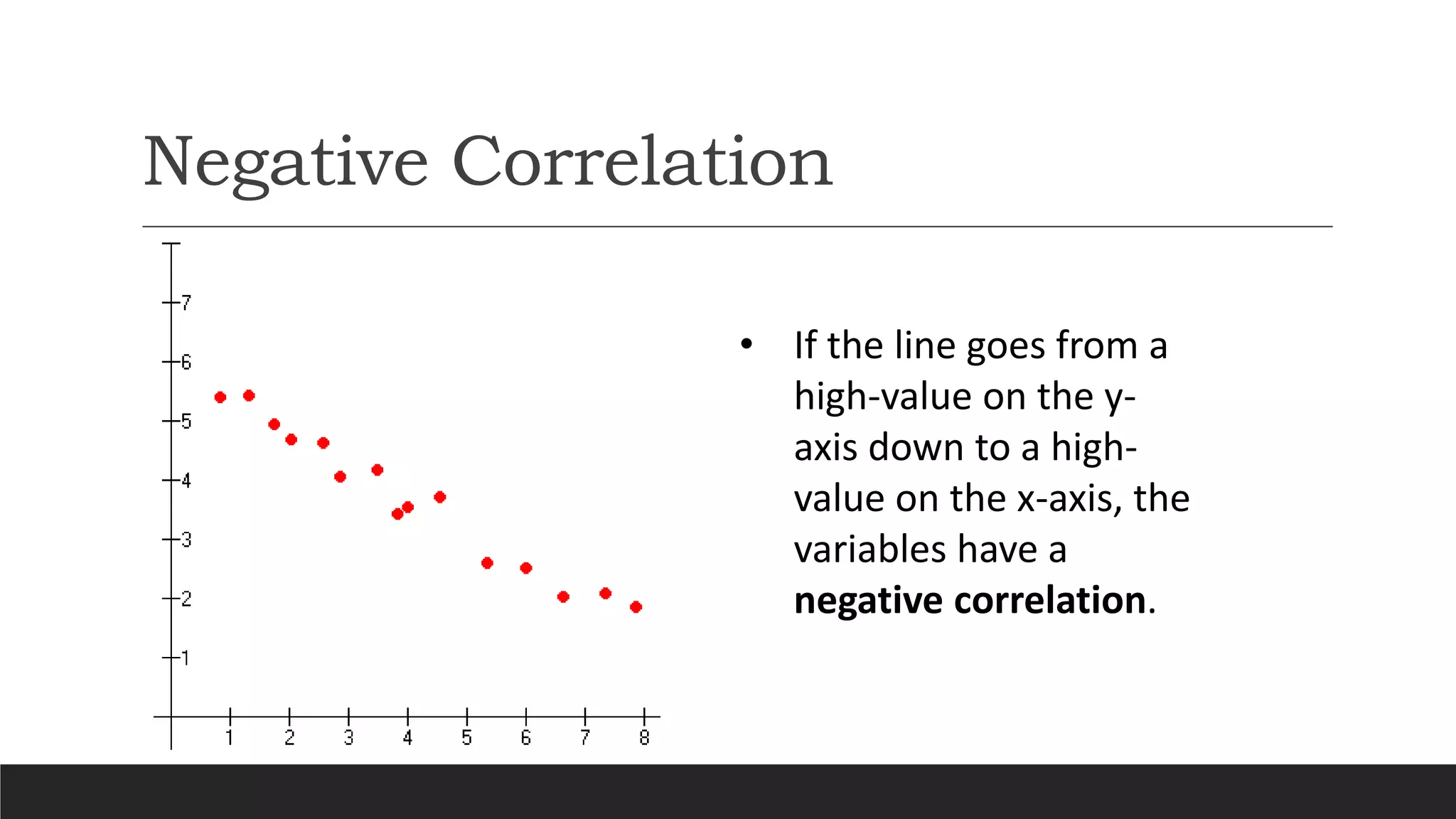
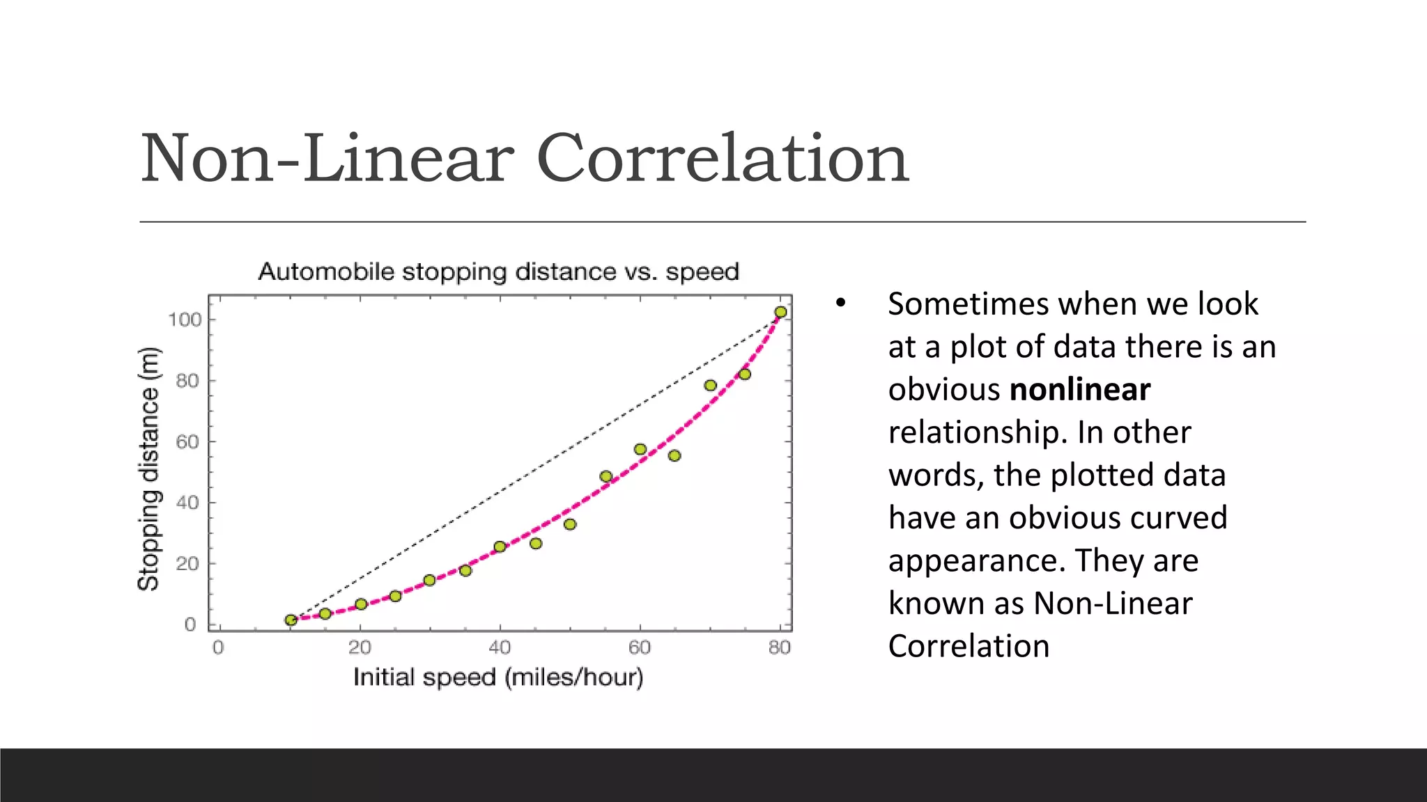
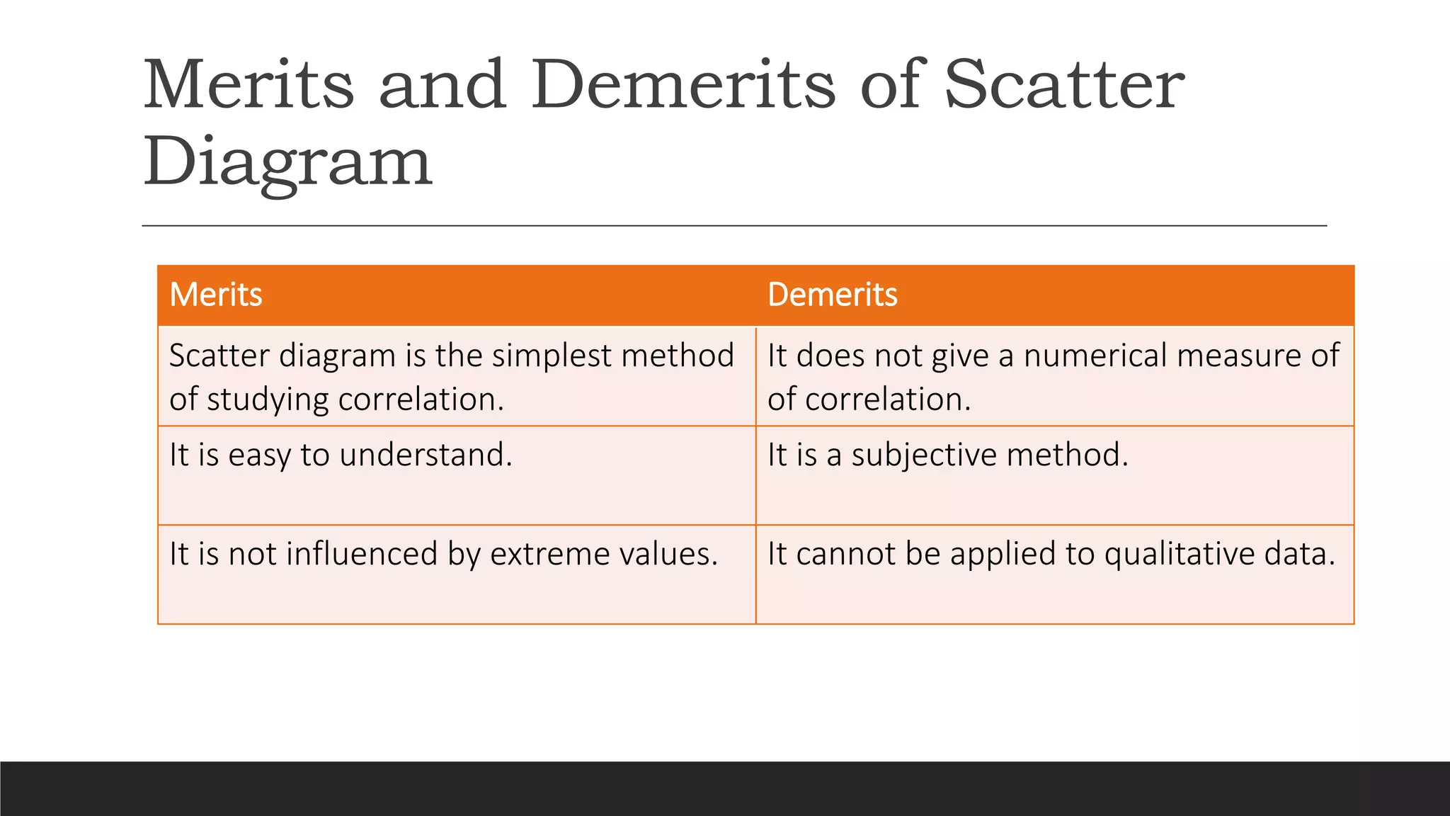
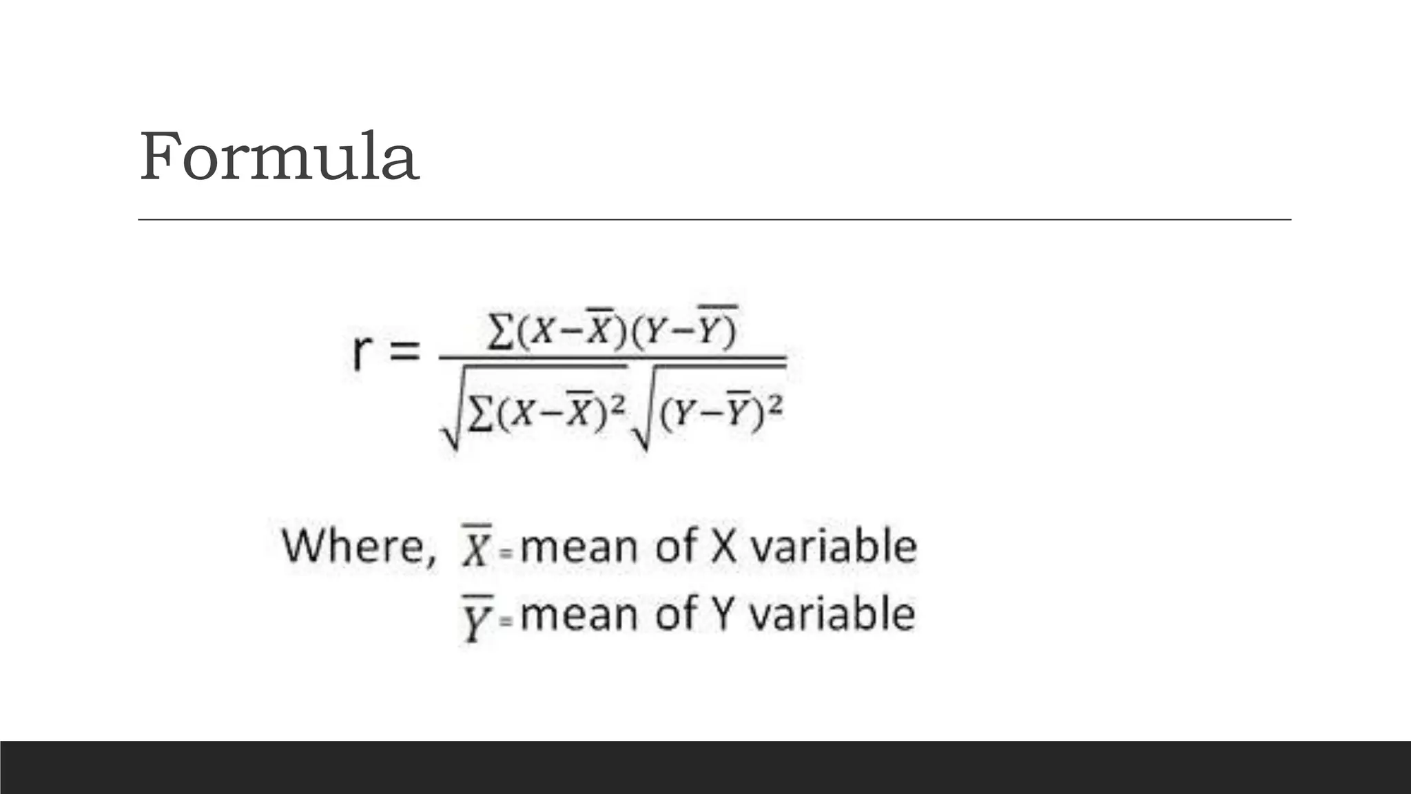
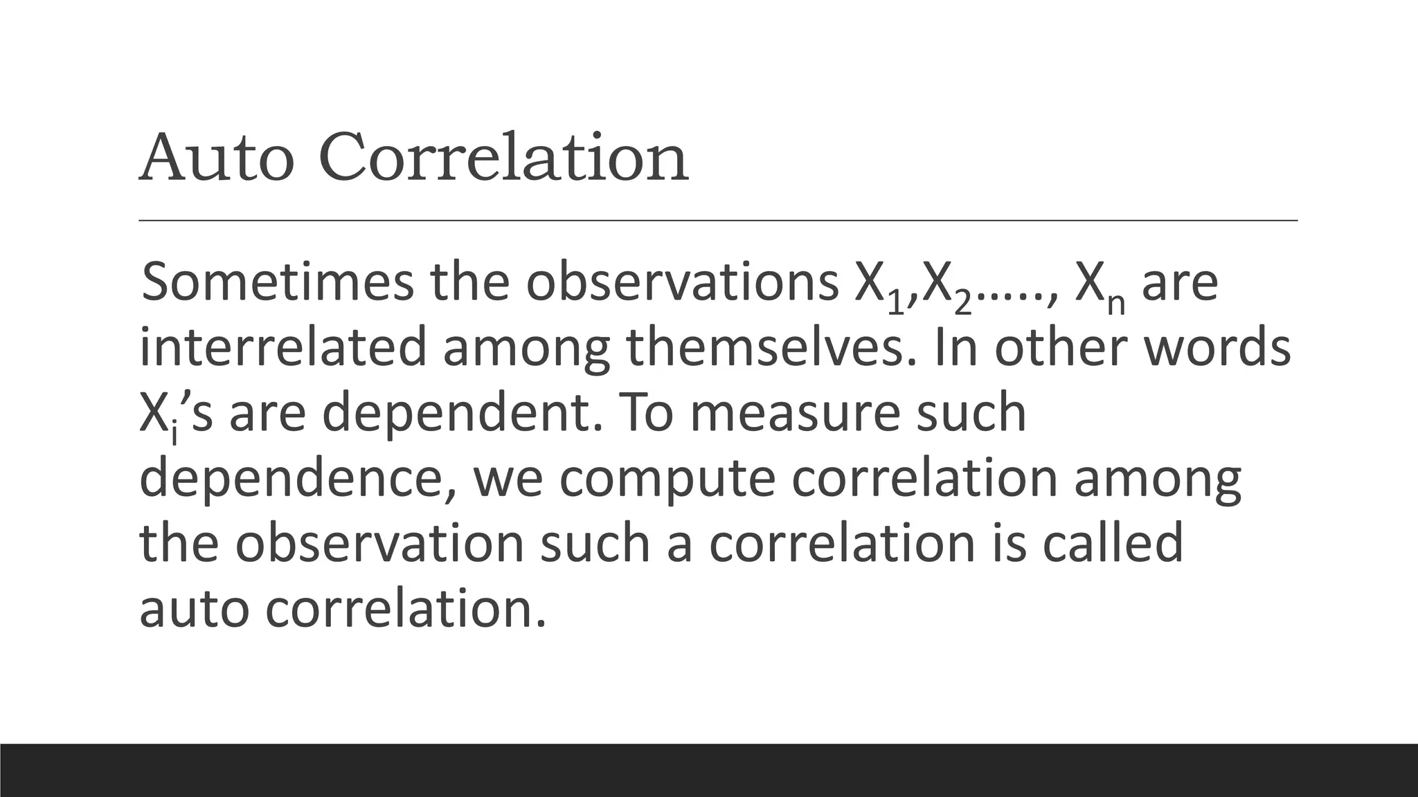
Correlation

Correlation
and types of
correlation.
JOSHUA RODRICK AND
MANAS PRADEEP

Introduction
Many a times we come across situations where two variables are interrelated.
For example:
◦ Marks and intelligence quotient of students.
◦ Demand and price of a certain commodity.
◦ Rainfall and agricultural production.
◦ Income and expenditure of a family.
In these situations we may be interested in examining the relation between the two variables.
Such interrelated variables are called as correlated variables.

Definition of Correlation and
Bivariate Data.
Correlation is a statistical tool to measure the extent of
linear relation between two variables.
Bivariate Data: In order to determine correlation, we
require data regarding two concerned variables. These data
are called bivariate data. Whenever the variables X and Y
are mentioned in the same item, they are likely to be
correlated.

Positive Correlation
In some cases, ↑Increase in value of one variable is
associated with ↑Increase in value of other variable or
↓Decrease in value of one variable is associated with
↓Decrease in value of other variable.
Correlation between these variables is said to be POSITIVE.

Negative Correlation
In some situations ↑Increase in value of one variable is
accompanied by ↓Decrease in value of other variable and
↓Decrease in value of one variable is accompanied by
↑Increase in value of the other Variable.
Correlation between these two variables is said to be
NEGATIVE.

Examples of Positive and Negative
Correlation
Positive Correlation Negative Correlation
Relationship between Sale of Cold
Drinks and Temperature.
Relationship between Alcohol
Consumption and Driving Ability.
Relationship Between DUI’s and
Accidents.
Relationship between Supply and price
of commodity.

No Correlation
In some cases change in one variable is not related to change in other
variable, In these cases there is said to be No Correlation or Zero
Correlation between the two variables.
For example,
◦ There is no relationship between the amount of tea drunk and level of
intelligence.
◦ There is no relationship between height of students and grades scored in
examinations.

Measures of Correlation
There are several measure of correlation some
of which are:
◦Scatter Diagram
◦Karl Pearson’s Coefficient of Correlation
◦Rank Correlation

Scatter Diagram
Scatter Diagram is a graph of observed
potted points where each points represents
the value of X & Y as a coordinate. It
portrays the relationship between these
two variables graphically.

Perfect Positive Correlation
• A perfect positive
correlation is given
the value of 1.

Perfect Negative Correlation
• A perfect negative
correlation is given
the value of -1.

Positive Correlation
• If the data points make a
straight line going from the
origin out to high x- and y-
values, then the variables
are said to have a positive
correlation.

Negative Correlation
• If the line goes from a
high-value on the y-
axis down to a high-
value on the x-axis, the
variables have a
negative correlation.

Non-Linear Correlation
• Sometimes when we look
at a plot of data there is an
obvious nonlinear
relationship. In other
words, the plotted data
have an obvious curved
appearance. They are
known as Non-Linear
Correlation

Merits and Demerits of Scatter
Diagram
Merits Demerits
Scatter diagram is the simplest method
of studying correlation.
It does not give a numerical measure of
of correlation.
It is easy to understand. It is a subjective method.
It is not influenced by extreme values. It cannot be applied to qualitative data.

Karl Pearson’s Coefficient of
correlation
oThe Karl Pearson’s correlation coefficient method is
quantitative and offers numerical value to establish the intensity
of linear relationship between X and Y.
oKarl Pearson’s coefficient correlation is represented by ‘r’.
oThe Pearson’s correlation measures the direction and degree of
linear relationship between two variables.

Merits and Demerits of Karl Pearson’s
Coefficient of Correlation
Merits Demerits
Karl Pearson’s coefficient of
correlation determines a single values
which summarizes the extent of linear
relationship. It also indicates types of
correlation.
It cannot be computed for qualitative
data such as honesty and intelligence,
beauty and intelligence.
It depends upon all observations. It is unduly affected by extreme
values.
It measures only linear relationship.

Applications of Karl Pearson’s
Coefficient of correlation
◦The Pearson correlation coefficient can be used
to summarize the strength of linear relationship
between two data samples.
◦The Pearson’s correlation coefficient is
calculated as the covariance of two variables
divided by the standard deviation of each data
sample.

Auto Correlation
Sometimes the observations X1,X2….., Xn are
interrelated among themselves. In other words
Xi’s are dependent. To measure such
dependence, we compute correlation among
the observation such a correlation is called
auto correlation.

Examples of Autocorrelation
◦During Monsoon, rainfall on nth day depends on rainfall on
(n-1)th Day or (n-2)th Day .
◦Price of share on nth day depends upon what happened on
earlier day or a few earlier days. In order to analyse the
data under this situation we make use of autocorrelation.
It has applications in the analysis of time series data.

Rank Correlation
◦Karl Pearson’s coefficient of correlation is the best
measure of correlation, however it poses difficulty in
measuring the correlation between qualitative
characteristics.
◦If the qualitative characteristics under study are recorded
using ordinal scale, we can arrange the items in ascending
or in descending order according to the merit that they
possess.

Rank Correlation
◦Ranking: Ordered arrangement if items according to merit
that they possess is called ranking.
◦Rank: The Number indicating the position in ranking is called
as rank.
◦Tie: Tie is said to occur in ranking if two or more items have
same merit. In this case we allot common rank to these items.
This rank is the average of ranks which would have been
allotted if the respective items would differ in merit slightly.

Rank Correlation
◦The product moment correlation between ranks is called
as Spearman’s rank correlation coefficient. It is
denoted by R.
◦R is a Karl Pearson’s coefficient of correlation for bivariate
data.

Rank Correlation
◦Spearman’s rank correlation is simple to compute as
compared t Karl Pearson’s coefficient of correlation. However
there is a loss of accuracy, whenever we compute it for
quantitative data.
◦Spearman’s rank correlation is most commonly used to
measure the correlation between the different traits such as
intelligence and mathematical aptitude.
◦Since R is Karl Pearson’s coefficient of correlation between the
ranks, it lies between -1 and 1.

Rank Correlation With Ties
oWhen ranking the data, ties(two or more
subjects having exactly the same value of a
variable) are likely to occur.
oIn case of ties, the tied observations receive the
same average rank.

oIf two or more items have same merit or quality, then
common rank is allotted to each of such items. This rank is
arithmetic mean of ranks which would have been given.
oIn case the corresponding items would differ slightly in
quality or merit. The number of items getting same rank
called as length of the tie.

oWe denote it by m. For example, suppose scores of the student
are to be ranked. Let the scores be arranged in increasing order.
oSupposed 3rd and 4th student have same scores, then we give
common rank to both. It will be an arithmetic mean of 3 and 4.
oHence, we give rank 3.5 to both the students. In this case length
of the tie is m = 2.

Thankyou.
JOSHUA RODRICK AND
MANAS PRADEEP

Correlation

More Related Content

What's hot

Similar to Correlation

Recently uploaded

Correlation