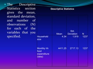
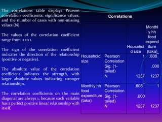
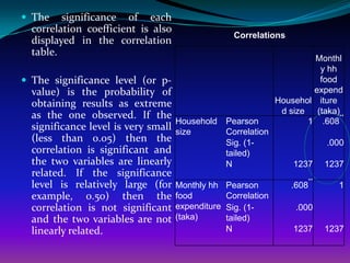
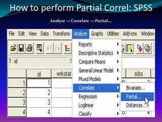
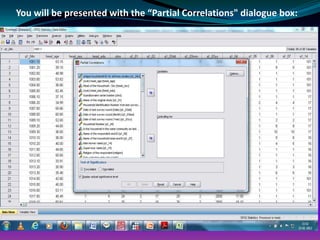
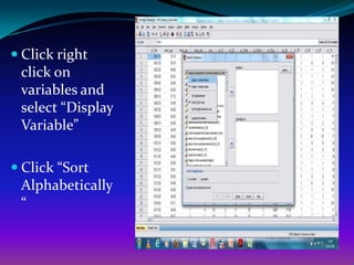
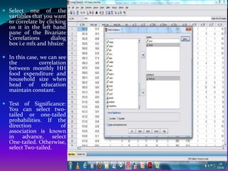
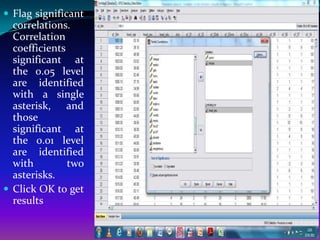
Srinivasulu Rajendran
 Centre for the Study of Regional Development (CSRD)


Jawaharlal Nehru University (JNU)
                      New Delhi
                        India
              r.srinivasulu@gmail.com
Objective of the session


          To understand
         CORRELATION
1. What is the procedure to
perform Correlation &
Regression?
2. How do we interpret results?
Identify the relationship between variables that
we want to perform Scatter plot for outliers and
type of relationship


 Monthly HH food Expenditure and HHSIZE
Interpreting Correlation Coefficient r


  strong correlation: r > .70 or r < –.70
  moderate correlation: r is between .30 & .70
      or r is between –.30 and –.70
  weak correlation: r is between 0 and .30
      or r is between 0 and –.30 .
GENERATE A SCATTERPLOT TO SEE
      THE RELATIONSHIPS
Go to Graphs → Legacy dialogues→ Scatter/Dot → Simple
       Click on DEPENDENT “mfx”. and move it to the Y-Axis
       Click on the “hhsize”. and move it to the X-Axis
Click OK
Scatterplot might not look promising at first
Double click on chart to open a CHART EDIT window
use Options →Bin Element   Simply CLOSE this box.
                           Bins are applied automatically.
BINS
Dot size now
       shows
  number of
  cases with
 each pair of
  X, Y values


  DO NOT CLOSE CHART EDITOR YET!
Add Fit Line (Regression)
 In Chart Editor:
 Elements
  →Fit Line at Total
 Close dialog box
  that opens
 Close Chart Editor
  window
Edited Scatterplot
 Distribution of
  cases shown by
  dots (bins)
 Trend shown
  by fit line.
Type of Correlation
 Bivariate Correlations.
 Partial Correlations
 Distances
BIVARIATE CORRELATIONS

 In Bivariate Correlations, the relationship between two
 variables is measured. The degree of relationship (how
 closely they are related) could be either positive or
 negative. The maximum number could be either +1
 (positive) or -1 (negative). This number is the
 correlation coefficient. A zero correlation indicates no
 relationship. Remember that you will want to perform
 a scatter plot before performing the correlation (to see
 if the assumptions have been met.)
Objective
 We are interested in whether an monthly HH food
 expenditure was correlated with hhsize.
Step 1
The Bivariate Correlations dialog box will appear
Right
 List of
              arrow
Variables
             button to
               add
             selected
            variable(s)
Step 2
 Select one of the variables that you want to correlate by
  clicking on it in the left hand pane of the Bivariate
  Correlations dialog box i.e mfx and hhsize
 Check the type of correlation coefficients that you require
  (Pearson for parametric, and Kendall’s tau-b and Spearman
  for non-parametric).
 Select the appropriate Test: Pearson’s correlation coefficient
  assumes that each pair of variables is bivariate normal and
  it is a measure of linear association. Two variables can be
  perfectly related, but if the relationship is not linear,
  Pearson’s correlation coefficient is not an appropriate
  statistic for measuring their association.
 Test of Significance: You can select two-tailed or one-tailed
  probabilities. If the direction of association is known in
  advance, select One-tailed. Otherwise, select Two-tailed.
 Flag significant correlations. Correlation coefficients
 significant at the 0.05 level are identified with a single
 asterisk, and those significant at the 0.01 level are
 identified with two asterisks.

 Click on the Options… button to select statistics, and
 select Means and SD and control the missing value by
 clicking “Exclude Cases pairwise.
Click on the Continue button.
Step 3
Click the OK button in
the Bivariate
Correlations dialog box
to run the analysis. The
output will be displayed
in a separate SPSS
Viewer window.
SPSS Output of Correlation Matrix
 The     Descriptive
 Statistics section                   Descriptive Statistics
 gives the mean,
 standard deviation,
 and number of
 observations (N)
 for each of the
                                                      Std.
 variables that you                        Mean     Deviation     N
 specified.             Household              4.34     1.919     1237
                        size


                        Monthly hh           4411.25    2717.13   1237
                        food
                        expenditure
                        (taka)
The correlations table displays Pearson
correlation coefficients, significance values,                  Correlations
and the number of cases with non-missing
values (N).
                                                                                    Monthl
                                                                                     y hh
The values of the correlation coefficient
                                                                                     food
range from -1 to 1.
                                                                                    expend
                                                                            Househol iture
The sign of the correlation coefficient
                                                                             d size (taka)
indicates the direction of the relationship Household         Pearson              1 .608
                                                                                           **
(positive or negative).                     size              Correlation
                                                              Sig. (1-                   .000
The absolute value of the correlation
                                                              tailed)
coefficient indicates the strength, with
                                                              N                 1237     1237
larger absolute values indicating stronger
relationships.                                                                      **
                                                Monthly hh    Pearson           .608       1
                                                food          Correlation
The correlation coefficients on the main
                                                expenditure   Sig. (1-           .000
diagonal are always 1, because each variable
                                                (taka)        tailed)
has a perfect positive linear relationship with
itself.                                                       N                 1237     1237
 The    significance of each
  correlation coefficient is also
                                                     Correlations
  displayed in the correlation
  table.
                                                                         Monthl
                                                                          y hh
 The significance level (or p-                                           food
  value) is the probability of                                           expend
  obtaining results as extreme                                   Househol iture
                                                                  d size (taka)
  as the one observed. If the                                                   **
                                     Household     Pearson              1 .608
  significance level is very small   size          Correlation
  (less than 0.05) then the                        Sig. (1-                   .000
  correlation is significant and                   tailed)
  the two variables are linearly                   N                 1237     1237
  related. If the significance
                                                                         **
  level is relatively large (for     Monthly hh    Pearson           .608       1
  example, 0.50) then the            food          Correlation
  correlation is not significant     expenditure   Sig. (1-           .000
  and the two variables are not      (taka)        tailed)
  linearly related.                                N                 1237     1237
Partial Correlations
 The Partial Correlations procedure computes partial
 correlation coefficients that describe the linear
 relationship between two variables while controlling
 for the effects of one or more additional variables.
 Correlations are measures of linear association. Two
 variables can be perfectly related, but if the
 relationship is not linear, a correlation coefficient is
 not a proper statistic to measure their association.
Step 1
How to perform Partial Correl: SPSS
         Analyze –> Correlate –> Partial...
You will be presented with the “Partial Correlations" dialogue box:
Step 2
 Click right
 click on
 variables and
 select “Display
 Variable”

 Click “Sort
 Alphabetically
 “
Step 3
Step 4
 Select one of the
  variables that you want
  to correlate by clicking
  on it in the left hand
  pane of the Bivariate
  Correlations      dialog
  box i.e mfx and hhsize

 In this case, we can see
  the          correlation
  between monthly HH
  food expenditure and
  household size when
  head of education
  maintain constant.

 Test of Significance:
  You can select two-
  tailed or one-tailed
  probabilities. If the
  direction          of
  association is known
  in advance, select
  One-tailed. Otherwise,
  select Two-tailed.
 Flag significant
  correlations.
  Correlation
  coefficients
  significant at
  the 0.05 level
  are identified
  with a single
  asterisk, and
  those
  significant at
  the 0.01 level
  are identified
  with         two
  asterisks.
 Click OK to get
  results
Step 5
As we can see, the                           Correlations

positive
                                                                           Monthl
correlation                                                                 y hh
                                                                            food
between mfx and                                                            expend
                                                                   Househol iture

hhsize        when    Control Variables
                      (sum) head_edu Household size Correlation
                                                                    d size (taka)
                                                                      1.000 .606

hh_edu           is                                 Significance          .   .000
                                                    (1-tailed)
maintained
constant         is                                 df                   0    1232


significant at 1%                    Monthly hh
                                     food
                                                    Correlation        .606 1.000


level (p > 0.00)                     expenditure
                                     (taka)
                                                    Significance
                                                    (1-tailed)
                                                                       .000      .


                                                    df                1232      0
Hands-on Exercises

 Find out the correlation       relationship between per
  capita total monthly expenditure and household size
  and identify the nature of relationship and define the
  reasons?
 Find out the correlation relationship between per
  capita total monthly expenditure and household size
  by controlling the village those who have adopted
  technology and not adopted tech?
 Find out the correlation relationship between per
  capita food expenditure and non-food expenditure by
  controlling district effect? [Hint: it is two tail why?]
Distances

 This procedure calculates any of a wide variety of
 statistics    measuring     either    similarities     or
 dissimilarities (distances), either between pairs of
 variables or between pairs of cases. These similarity or
 distance measures can then be used with other
 procedures, such as factor analysis, cluster analysis, or
 multidimensional scaling, to help analyze complex
 data sets.

Topic 15 correlation spss

  • 1.
    Srinivasulu Rajendran Centrefor the Study of Regional Development (CSRD) Jawaharlal Nehru University (JNU) New Delhi India r.srinivasulu@gmail.com
  • 2.
    Objective of thesession To understand CORRELATION
  • 3.
    1. What isthe procedure to perform Correlation & Regression? 2. How do we interpret results?
  • 4.
    Identify the relationshipbetween variables that we want to perform Scatter plot for outliers and type of relationship  Monthly HH food Expenditure and HHSIZE
  • 5.
    Interpreting Correlation Coefficientr  strong correlation: r > .70 or r < –.70  moderate correlation: r is between .30 & .70 or r is between –.30 and –.70  weak correlation: r is between 0 and .30 or r is between 0 and –.30 .
  • 6.
    GENERATE A SCATTERPLOTTO SEE THE RELATIONSHIPS Go to Graphs → Legacy dialogues→ Scatter/Dot → Simple Click on DEPENDENT “mfx”. and move it to the Y-Axis Click on the “hhsize”. and move it to the X-Axis Click OK
  • 7.
    Scatterplot might notlook promising at first Double click on chart to open a CHART EDIT window
  • 8.
    use Options →BinElement Simply CLOSE this box. Bins are applied automatically.
  • 9.
    BINS Dot size now shows number of cases with each pair of X, Y values DO NOT CLOSE CHART EDITOR YET!
  • 10.
    Add Fit Line(Regression)  In Chart Editor:  Elements →Fit Line at Total  Close dialog box that opens  Close Chart Editor window
  • 11.
    Edited Scatterplot  Distributionof cases shown by dots (bins)  Trend shown by fit line.
  • 12.
    Type of Correlation Bivariate Correlations.  Partial Correlations  Distances
  • 13.
    BIVARIATE CORRELATIONS  InBivariate Correlations, the relationship between two variables is measured. The degree of relationship (how closely they are related) could be either positive or negative. The maximum number could be either +1 (positive) or -1 (negative). This number is the correlation coefficient. A zero correlation indicates no relationship. Remember that you will want to perform a scatter plot before performing the correlation (to see if the assumptions have been met.)
  • 14.
    Objective  We areinterested in whether an monthly HH food expenditure was correlated with hhsize.
  • 15.
  • 17.
    The Bivariate Correlationsdialog box will appear
  • 18.
    Right List of arrow Variables button to add selected variable(s)
  • 19.
  • 20.
     Select oneof the variables that you want to correlate by clicking on it in the left hand pane of the Bivariate Correlations dialog box i.e mfx and hhsize  Check the type of correlation coefficients that you require (Pearson for parametric, and Kendall’s tau-b and Spearman for non-parametric).  Select the appropriate Test: Pearson’s correlation coefficient assumes that each pair of variables is bivariate normal and it is a measure of linear association. Two variables can be perfectly related, but if the relationship is not linear, Pearson’s correlation coefficient is not an appropriate statistic for measuring their association.  Test of Significance: You can select two-tailed or one-tailed probabilities. If the direction of association is known in advance, select One-tailed. Otherwise, select Two-tailed.
  • 21.
     Flag significantcorrelations. Correlation coefficients significant at the 0.05 level are identified with a single asterisk, and those significant at the 0.01 level are identified with two asterisks.  Click on the Options… button to select statistics, and select Means and SD and control the missing value by clicking “Exclude Cases pairwise.
  • 22.
    Click on theContinue button.
  • 23.
  • 24.
    Click the OKbutton in the Bivariate Correlations dialog box to run the analysis. The output will be displayed in a separate SPSS Viewer window.
  • 25.
    SPSS Output ofCorrelation Matrix
  • 26.
     The Descriptive Statistics section Descriptive Statistics gives the mean, standard deviation, and number of observations (N) for each of the Std. variables that you Mean Deviation N specified. Household 4.34 1.919 1237 size Monthly hh 4411.25 2717.13 1237 food expenditure (taka)
  • 27.
    The correlations tabledisplays Pearson correlation coefficients, significance values, Correlations and the number of cases with non-missing values (N). Monthl y hh The values of the correlation coefficient food range from -1 to 1. expend Househol iture The sign of the correlation coefficient d size (taka) indicates the direction of the relationship Household Pearson 1 .608 ** (positive or negative). size Correlation Sig. (1- .000 The absolute value of the correlation tailed) coefficient indicates the strength, with N 1237 1237 larger absolute values indicating stronger relationships. ** Monthly hh Pearson .608 1 food Correlation The correlation coefficients on the main expenditure Sig. (1- .000 diagonal are always 1, because each variable (taka) tailed) has a perfect positive linear relationship with itself. N 1237 1237
  • 28.
     The significance of each correlation coefficient is also Correlations displayed in the correlation table. Monthl y hh  The significance level (or p- food value) is the probability of expend obtaining results as extreme Househol iture d size (taka) as the one observed. If the ** Household Pearson 1 .608 significance level is very small size Correlation (less than 0.05) then the Sig. (1- .000 correlation is significant and tailed) the two variables are linearly N 1237 1237 related. If the significance ** level is relatively large (for Monthly hh Pearson .608 1 example, 0.50) then the food Correlation correlation is not significant expenditure Sig. (1- .000 and the two variables are not (taka) tailed) linearly related. N 1237 1237
  • 29.
    Partial Correlations  ThePartial Correlations procedure computes partial correlation coefficients that describe the linear relationship between two variables while controlling for the effects of one or more additional variables. Correlations are measures of linear association. Two variables can be perfectly related, but if the relationship is not linear, a correlation coefficient is not a proper statistic to measure their association.
  • 30.
  • 31.
    How to performPartial Correl: SPSS Analyze –> Correlate –> Partial...
  • 32.
    You will bepresented with the “Partial Correlations" dialogue box:
  • 33.
  • 34.
     Click right click on variables and select “Display Variable”  Click “Sort Alphabetically “
  • 35.
  • 37.
  • 38.
     Select oneof the variables that you want to correlate by clicking on it in the left hand pane of the Bivariate Correlations dialog box i.e mfx and hhsize  In this case, we can see the correlation between monthly HH food expenditure and household size when head of education maintain constant.  Test of Significance: You can select two- tailed or one-tailed probabilities. If the direction of association is known in advance, select One-tailed. Otherwise, select Two-tailed.
  • 39.
     Flag significant correlations. Correlation coefficients significant at the 0.05 level are identified with a single asterisk, and those significant at the 0.01 level are identified with two asterisks.  Click OK to get results
  • 40.
  • 41.
    As we cansee, the Correlations positive Monthl correlation y hh food between mfx and expend Househol iture hhsize when Control Variables (sum) head_edu Household size Correlation d size (taka) 1.000 .606 hh_edu is Significance . .000 (1-tailed) maintained constant is df 0 1232 significant at 1% Monthly hh food Correlation .606 1.000 level (p > 0.00) expenditure (taka) Significance (1-tailed) .000 . df 1232 0
  • 42.
    Hands-on Exercises  Findout the correlation relationship between per capita total monthly expenditure and household size and identify the nature of relationship and define the reasons?  Find out the correlation relationship between per capita total monthly expenditure and household size by controlling the village those who have adopted technology and not adopted tech?  Find out the correlation relationship between per capita food expenditure and non-food expenditure by controlling district effect? [Hint: it is two tail why?]
  • 43.
    Distances  This procedurecalculates any of a wide variety of statistics measuring either similarities or dissimilarities (distances), either between pairs of variables or between pairs of cases. These similarity or distance measures can then be used with other procedures, such as factor analysis, cluster analysis, or multidimensional scaling, to help analyze complex data sets.