02 data

1
Data Mining
— Chapter 2 —
สอนโดย
อาจารย์ หทัยรัตน์ เกตุมณีชัยรัตน์
ภาควิชาการจัดการเทคโนโลยีการผลิตและสารสนเทศ

2
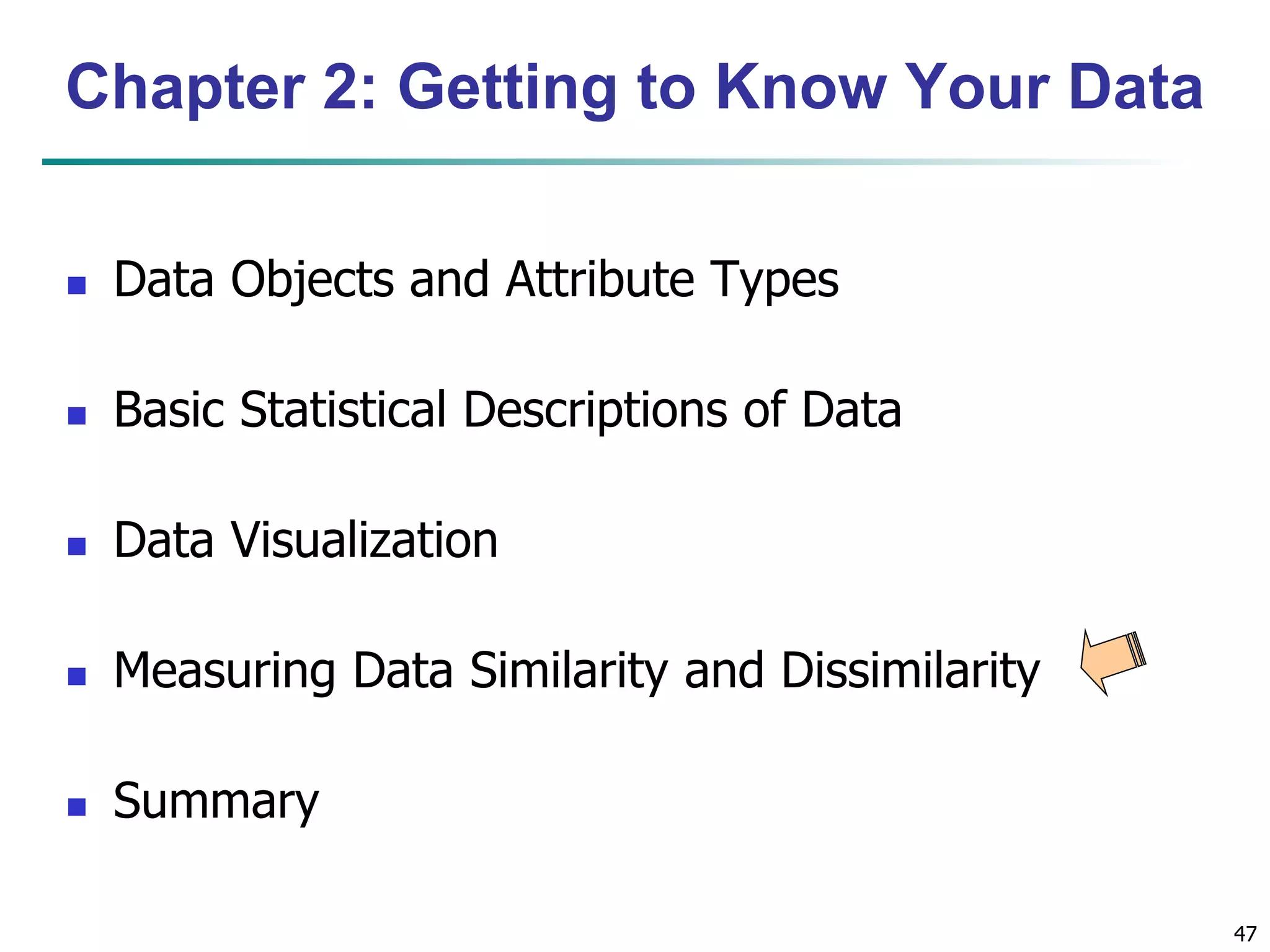
Chapter 2: Getting to Know Your Data
 Data Objects and Attribute Types
 Basic Statistical Descriptions of Data
 Data Visualization
 Measuring Data Similarity and Dissimilarity
 Summary

3
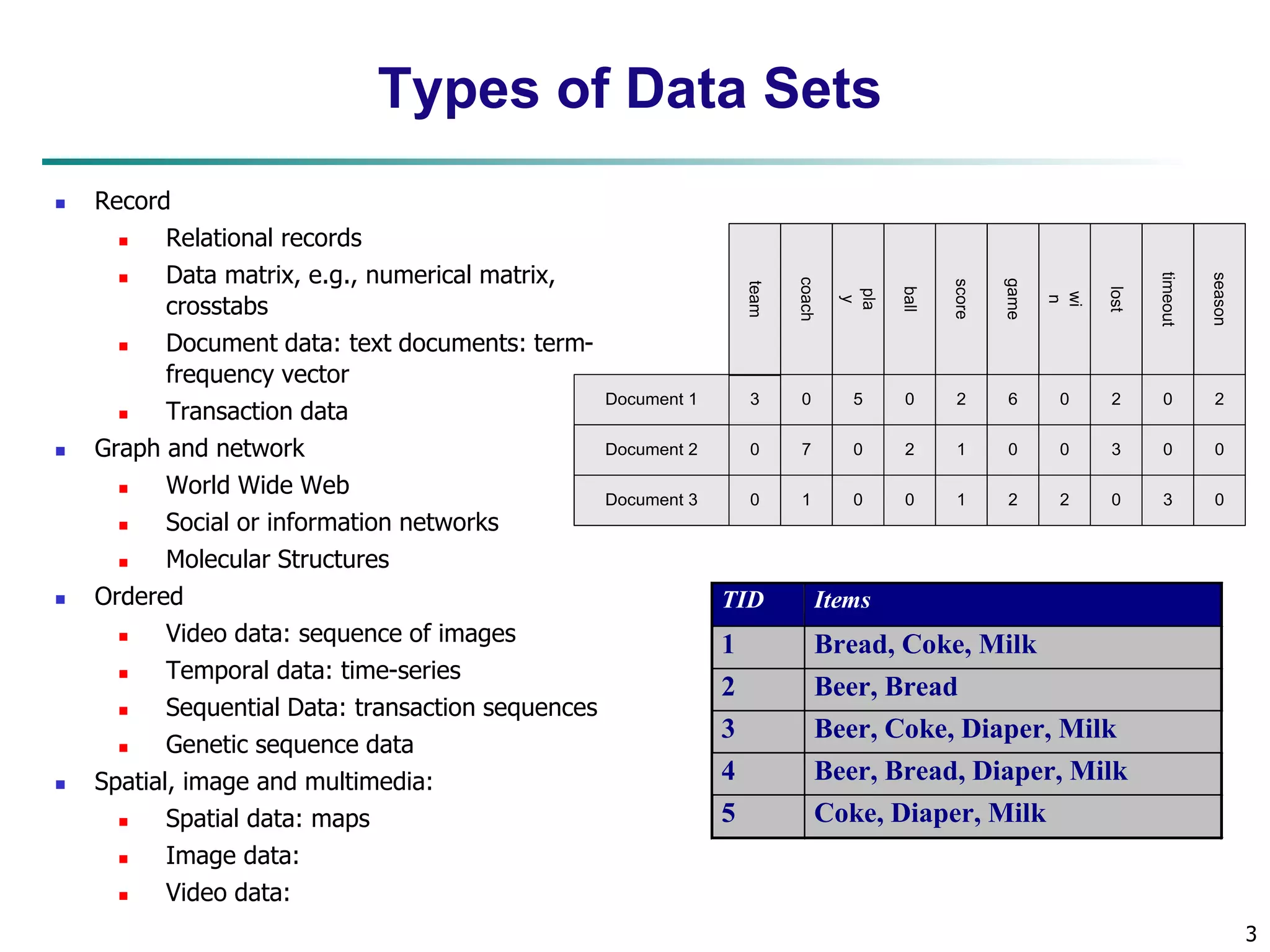
Types of Data Sets
 Record
 Relational records
 Data matrix, e.g., numerical matrix,
crosstabs
 Document data: text documents: term-frequency
vector
 Transaction data
 Graph and network
 World Wide Web
 Social or information networks
 Molecular Structures
 Ordered
 Video data: sequence of images
 Temporal data: time-series
 Sequential Data: transaction sequences
 Genetic sequence data
 Spatial, image and multimedia:
 Spatial data: maps
 Image data:
 Video data:
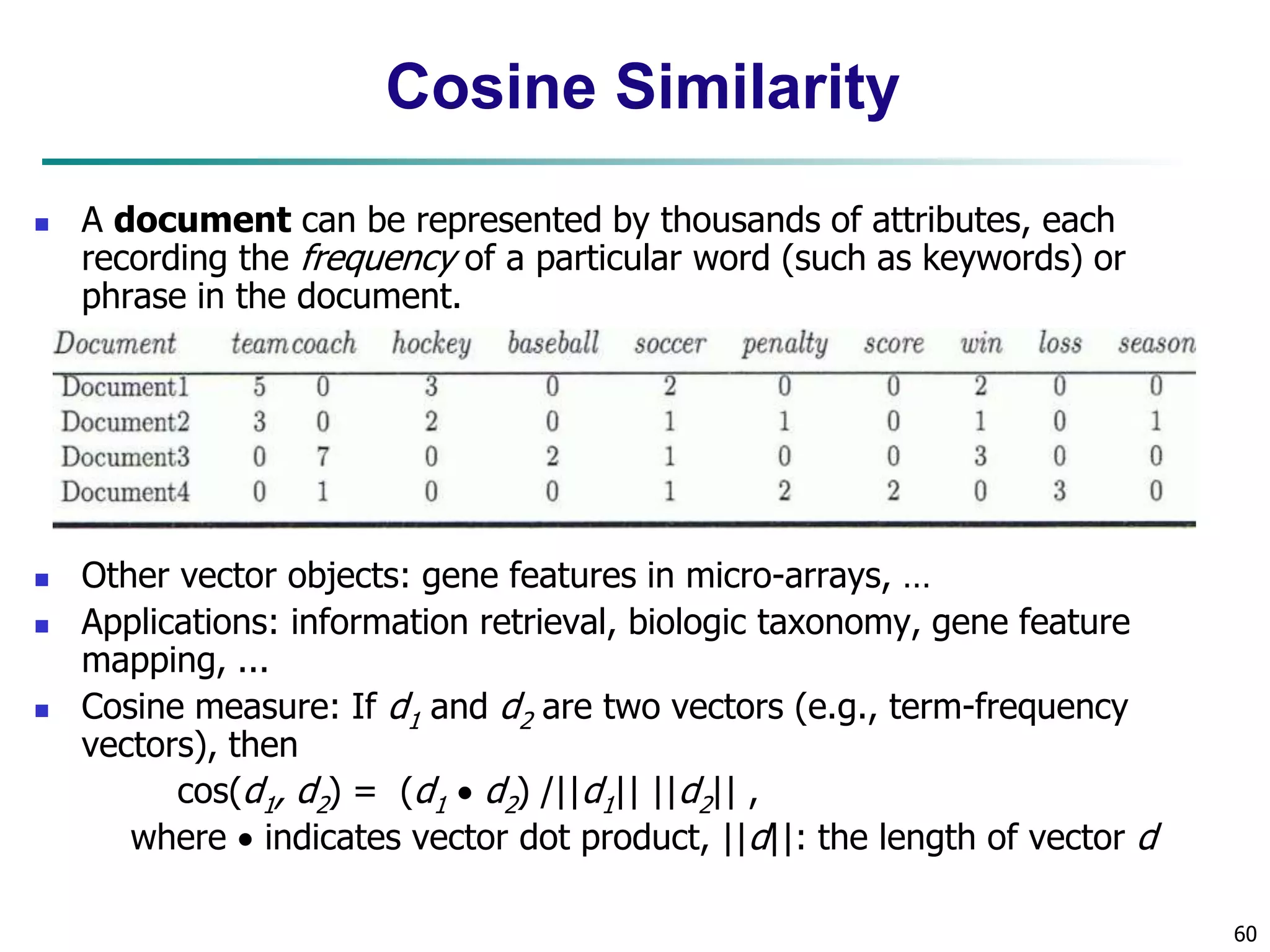
Document 1
season
timeout
lost
wi
n
game
score
ball
pla
y
coach
team
Document 2
Document 3
3 0 5 0 2 6 0 2 0 2
0
0
7 0 2 1 0 0 3 0 0
1 0 0 1 2 2 0 3 0
TID Items
1 Bread, Coke, Milk
2 Beer, Bread
3 Beer, Coke, Diaper, Milk
4 Beer, Bread, Diaper, Milk
5 Coke, Diaper, Milk

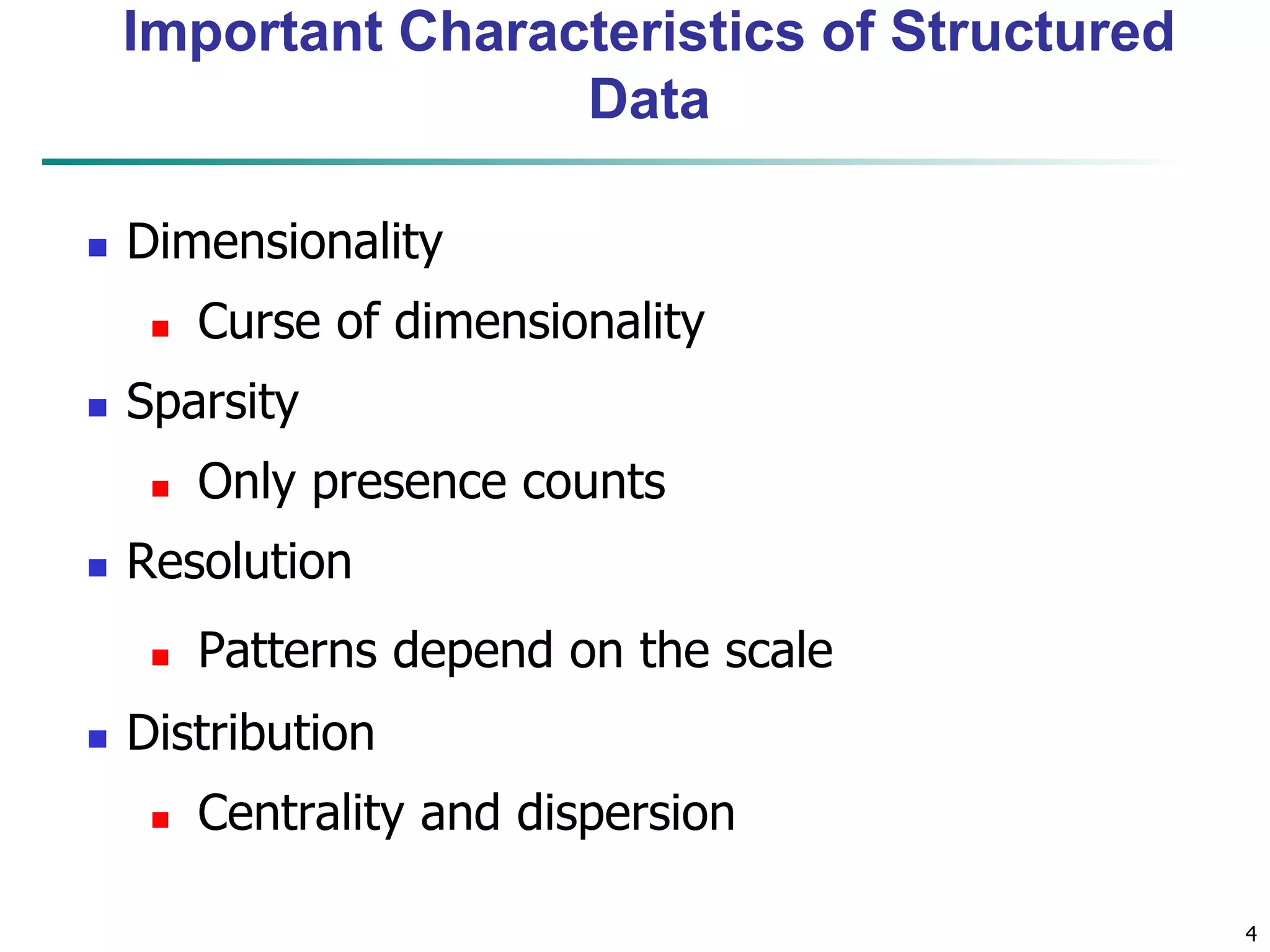
4
Important Characteristics of Structured
Data
 Dimensionality
 Curse of dimensionality
 Sparsity
 Only presence counts
 Resolution
 Patterns depend on the scale
 Distribution
 Centrality and dispersion

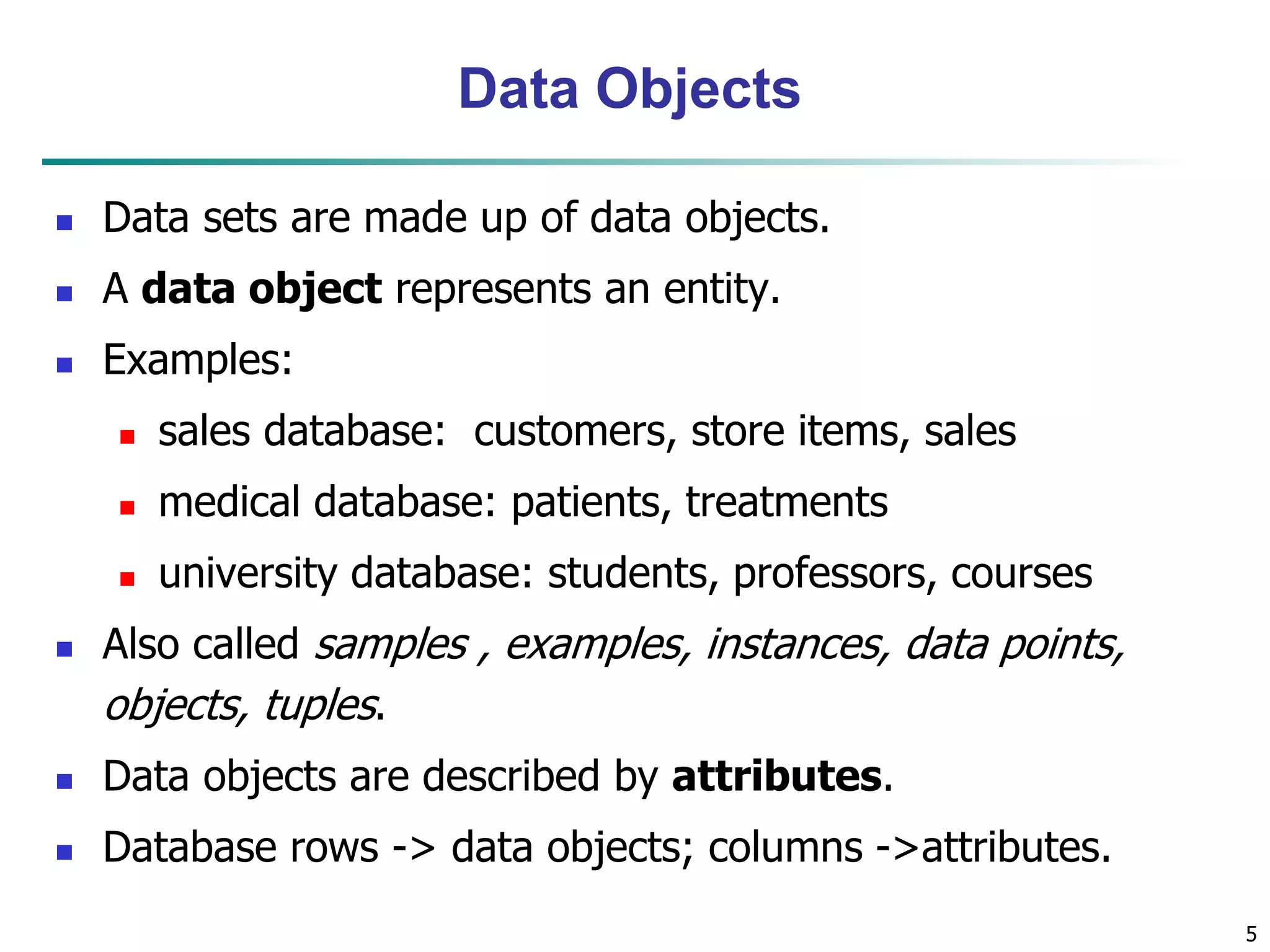
5
Data Objects
 Data sets are made up of data objects.
 A data object represents an entity.
 Examples:
 sales database: customers, store items, sales
 medical database: patients, treatments
 university database: students, professors, courses
 Also called samples , examples, instances, data points,
objects, tuples.
 Data objects are described by attributes.
 Database rows -> data objects; columns ->attributes.

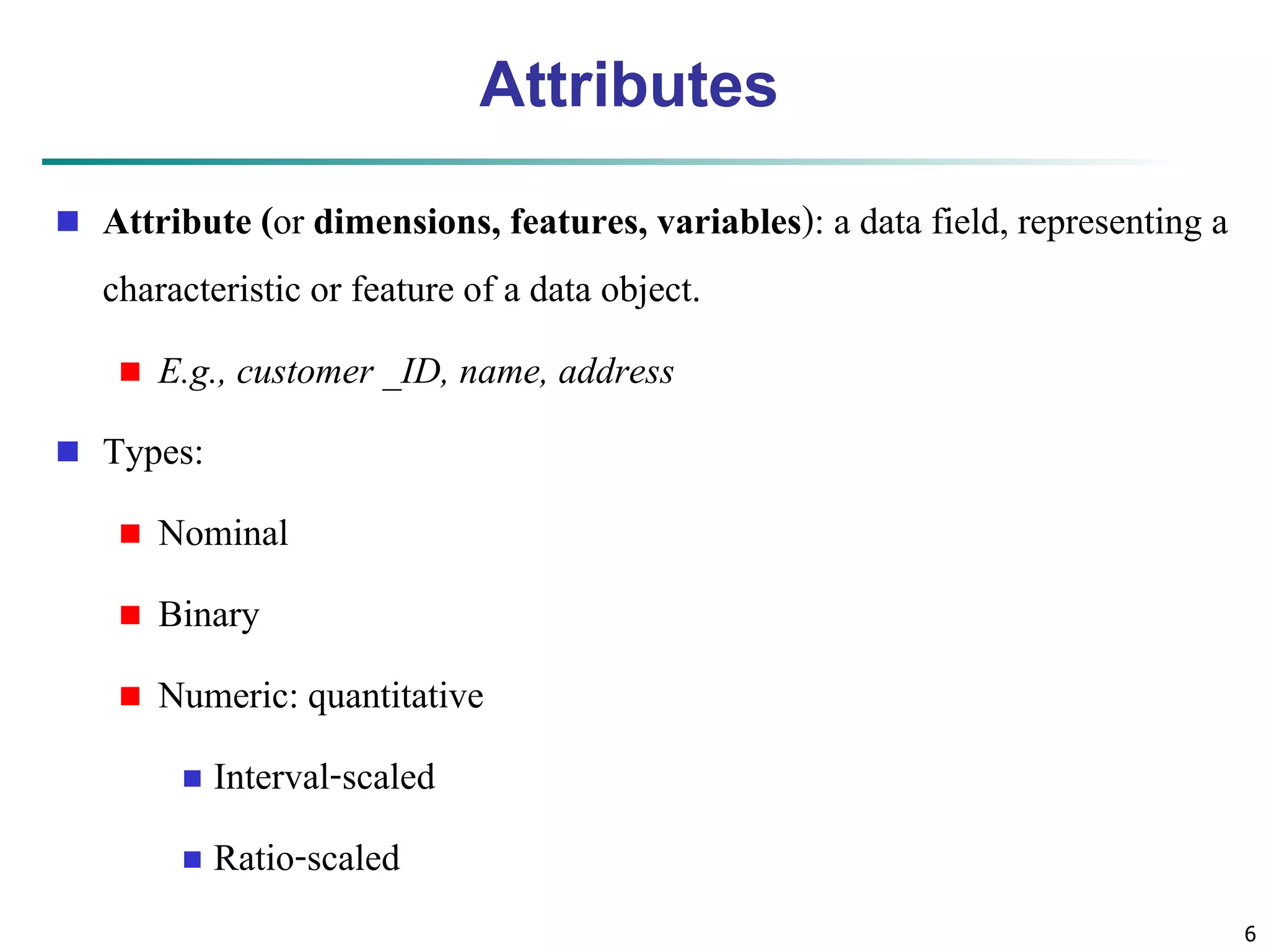
6
Attributes
 Attribute (or dimensions, features, variables): a data field, representing a
characteristic or feature of a data object.
 E.g., customer _ID, name, address
 Types:
 Nominal
 Binary
 Numeric: quantitative
 Interval-scaled
 Ratio-scaled

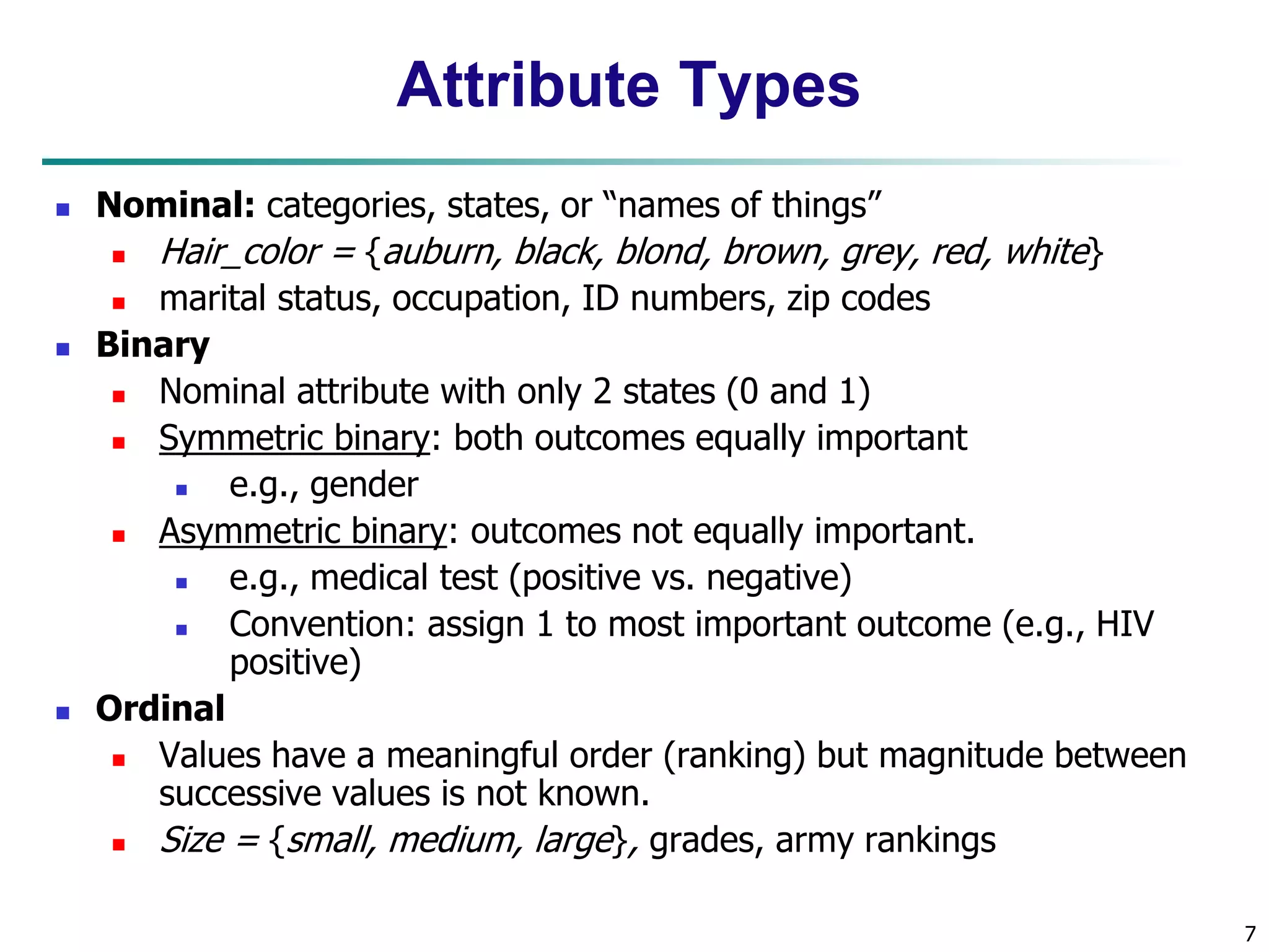
7
Attribute Types
 Nominal: categories, states, or “names of things”
 Hair_color = {auburn, black, blond, brown, grey, red, white}
 marital status, occupation, ID numbers, zip codes
 Binary
 Nominal attribute with only 2 states (0 and 1)
 Symmetric binary: both outcomes equally important
 e.g., gender
 Asymmetric binary: outcomes not equally important.
 e.g., medical test (positive vs. negative)
 Convention: assign 1 to most important outcome (e.g., HIV
positive)
 Ordinal
 Values have a meaningful order (ranking) but magnitude between
successive values is not known.
 Size = {small, medium, large}, grades, army rankings

8
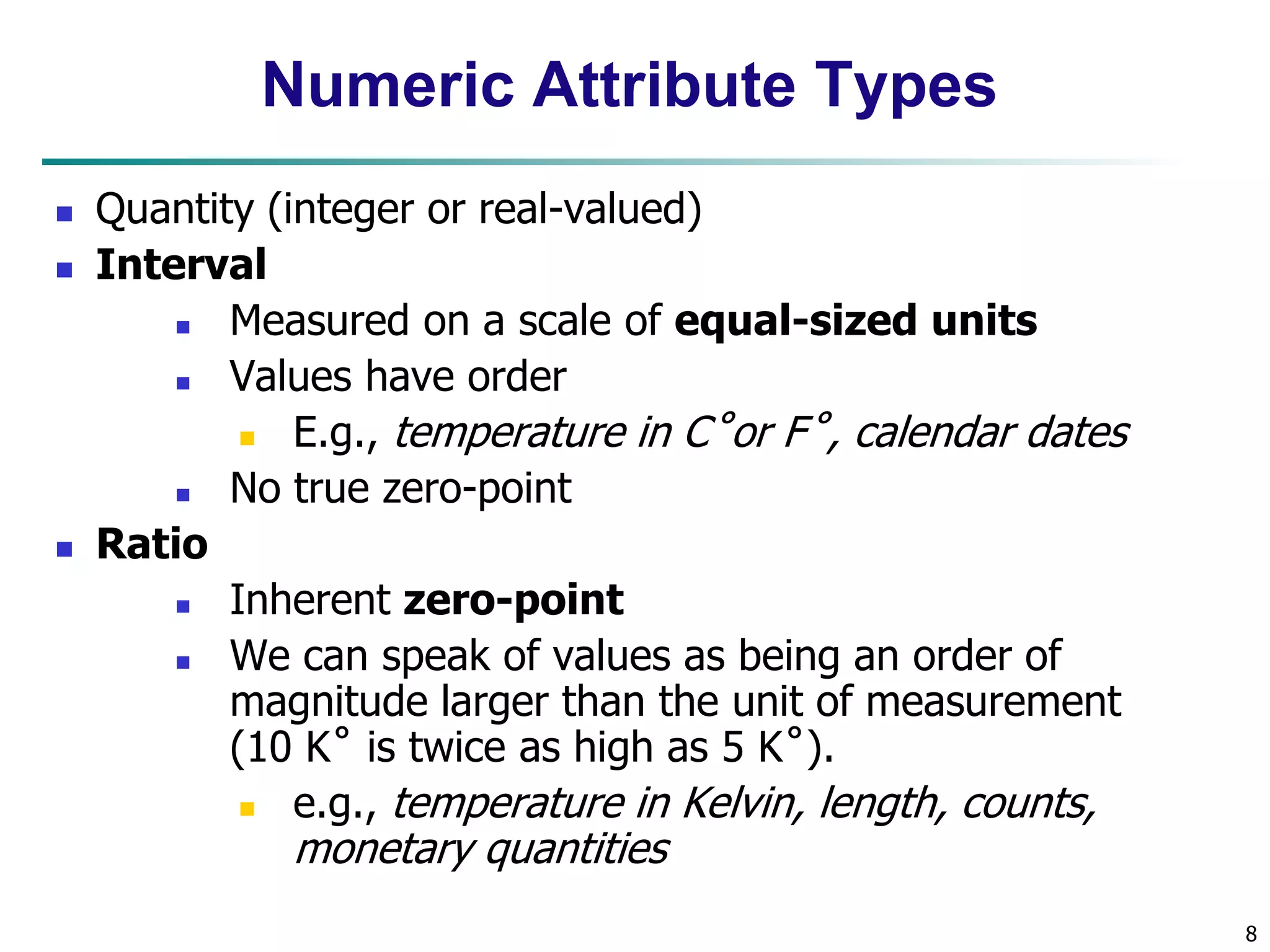
Numeric Attribute Types
 Quantity (integer or real-valued)
 Interval
 Measured on a scale of equal-sized units
 Values have order
 E.g., temperature in C˚or F˚, calendar dates
 No true zero-point
 Ratio
 Inherent zero-point
 We can speak of values as being an order of
magnitude larger than the unit of measurement
(10 K˚ is twice as high as 5 K˚).
 e.g., temperature in Kelvin, length, counts,
monetary quantities

9
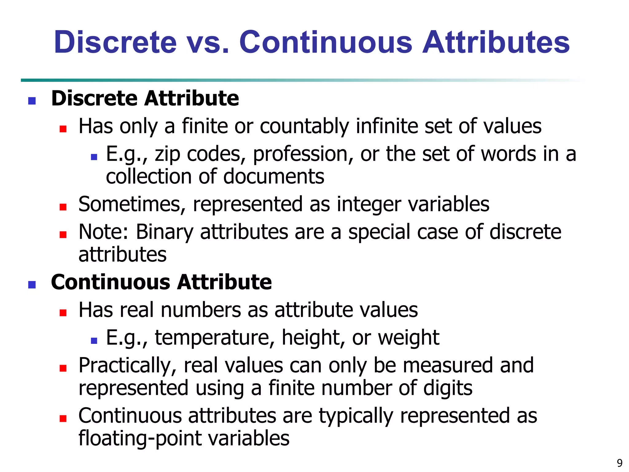
Discrete vs. Continuous Attributes
 Discrete Attribute
 Has only a finite or countably infinite set of values
 E.g., zip codes, profession, or the set of words in a
collection of documents
 Sometimes, represented as integer variables
 Note: Binary attributes are a special case of discrete
attributes
 Continuous Attribute
 Has real numbers as attribute values
 E.g., temperature, height, or weight
 Practically, real values can only be measured and
represented using a finite number of digits
 Continuous attributes are typically represented as
floating-point variables

10
 Summary

11
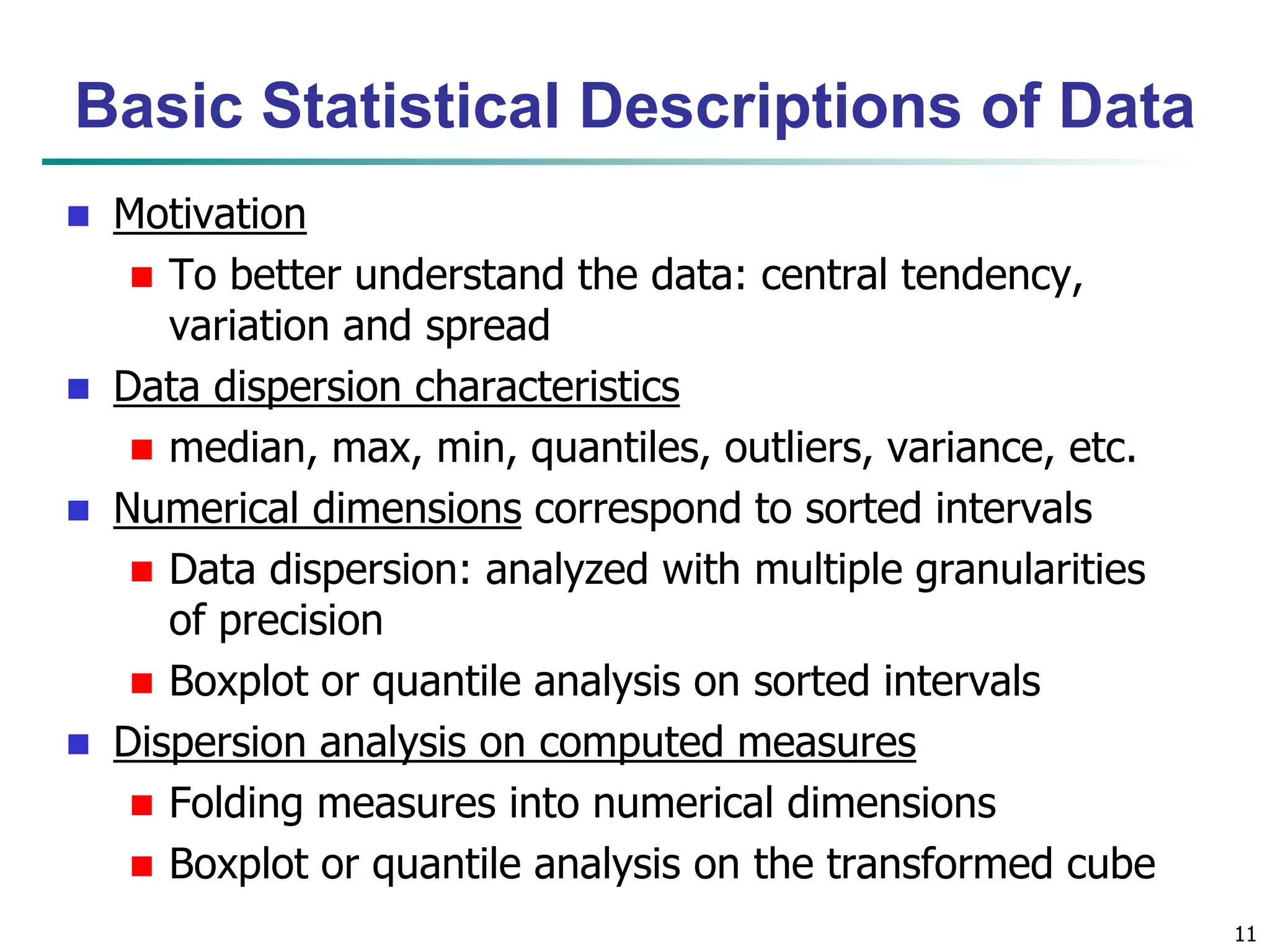
Basic Statistical Descriptions of Data
 Motivation
 To better understand the data: central tendency,
variation and spread
 Data dispersion characteristics
 median, max, min, quantiles, outliers, variance, etc.
 Numerical dimensions correspond to sorted intervals
 Data dispersion: analyzed with multiple granularities
of precision
 Boxplot or quantile analysis on sorted intervals
 Dispersion analysis on computed measures
 Folding measures into numerical dimensions
 Boxplot or quantile analysis on the transformed cube

x   
12
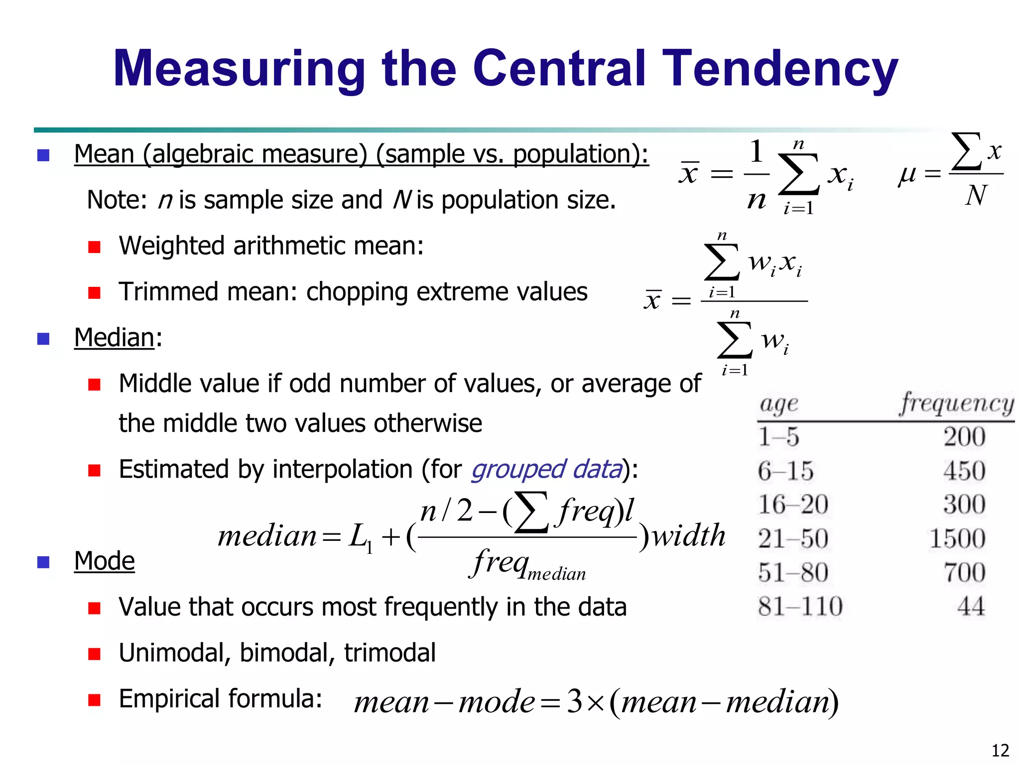
Measuring the Central Tendency
 Mean (algebraic measure) (sample vs. population):
Note: n is sample size and N is population size.
 Weighted arithmetic mean:
 Trimmed mean: chopping extreme values
 Median:
  n
 Middle value if odd number of values, or average of
the middle two values otherwise
 Estimated by interpolation (for grouped data):
 Mode
n freq l
 Value that occurs most frequently in the data
 Unimodal, bimodal, trimodal
 Empirical formula:



n
i
i x
n
x
1
1

w x


i
i
n
i
i i
w
x
1
1
width
freq
median L
median
)
/ 2 ( )
( 1
 
 
meanmode  3(meanmedian)
N

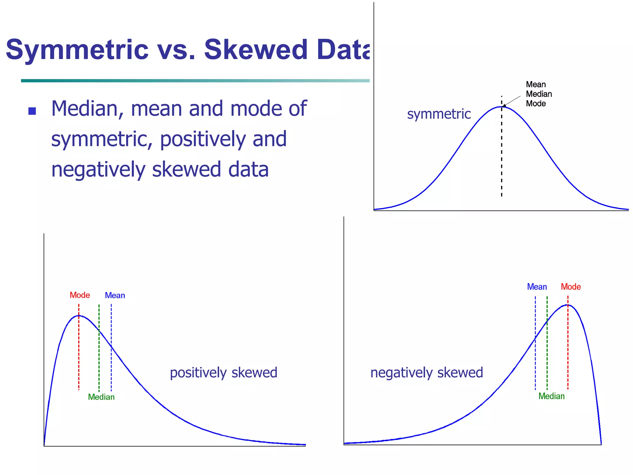
Symmetric vs. Skewed Data
 Median, mean and mode of
symmetric, positively and
negatively skewed data
symmetric
positively skewed negatively skewed
November 20, 2014 Data Mining: Concepts and Techniques 13

14
Measuring the Dispersion of Data
 Quartiles, outliers and boxplots
 Quartiles: Q1 (25th percentile), Q3 (75th percentile)
 Inter-quartile range: IQR = Q3 – Q1
 Five number summary: min, Q1, median, Q3, max
 Boxplot: ends of the box are the quartiles; median is marked; add
whiskers, and plot outliers individually
 Outlier: usually, a value higher/lower than 1.5 x IQR
 Variance and standard deviation (sample: s, population: σ)
 Variance: (algebraic, scalable computation)
2 2
2 2 ( ) ]
  
 


  

i i
n
2 2 1
 Standard deviation s (or σ) is the square root of variance s2 (or σ2)

n
i
n
i
n
i
i x
n
x
n
x x
n
s
1 1
1
1
[
1
1
( )
1
1
 
 
   
i
i
n
i
i x
N
x
N 1
2 2
1
( )
1
  

15
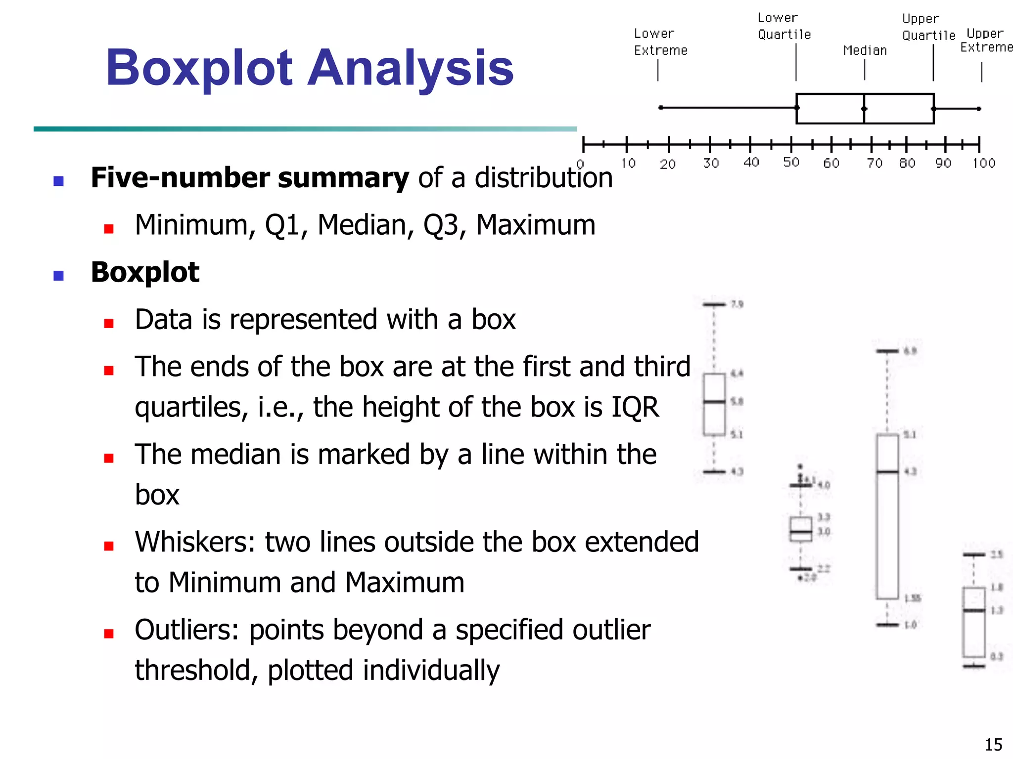
Boxplot Analysis
 Five-number summary of a distribution
 Minimum, Q1, Median, Q3, Maximum
 Boxplot
 Data is represented with a box
 The ends of the box are at the first and third
quartiles, i.e., the height of the box is IQR
 The median is marked by a line within the
box
 Whiskers: two lines outside the box extended
to Minimum and Maximum
 Outliers: points beyond a specified outlier
threshold, plotted individually

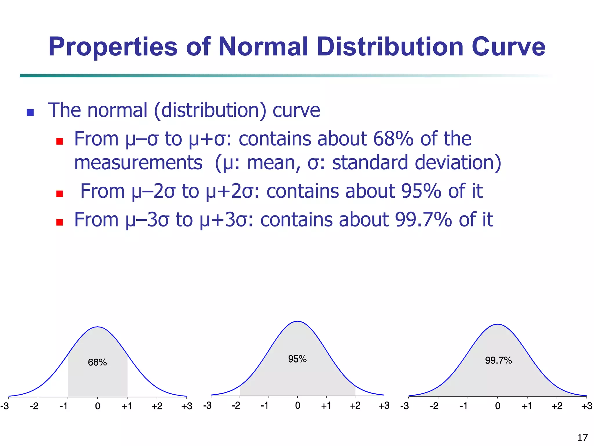
Visualization of Data Dispersion: 3-D Boxplots
16

17
Properties of Normal Distribution Curve
 The normal (distribution) curve
 From μ–σ to μ+σ: contains about 68% of the
measurements (μ: mean, σ: standard deviation)
 From μ–2σ to μ+2σ: contains about 95% of it
 From μ–3σ to μ+3σ: contains about 99.7% of it

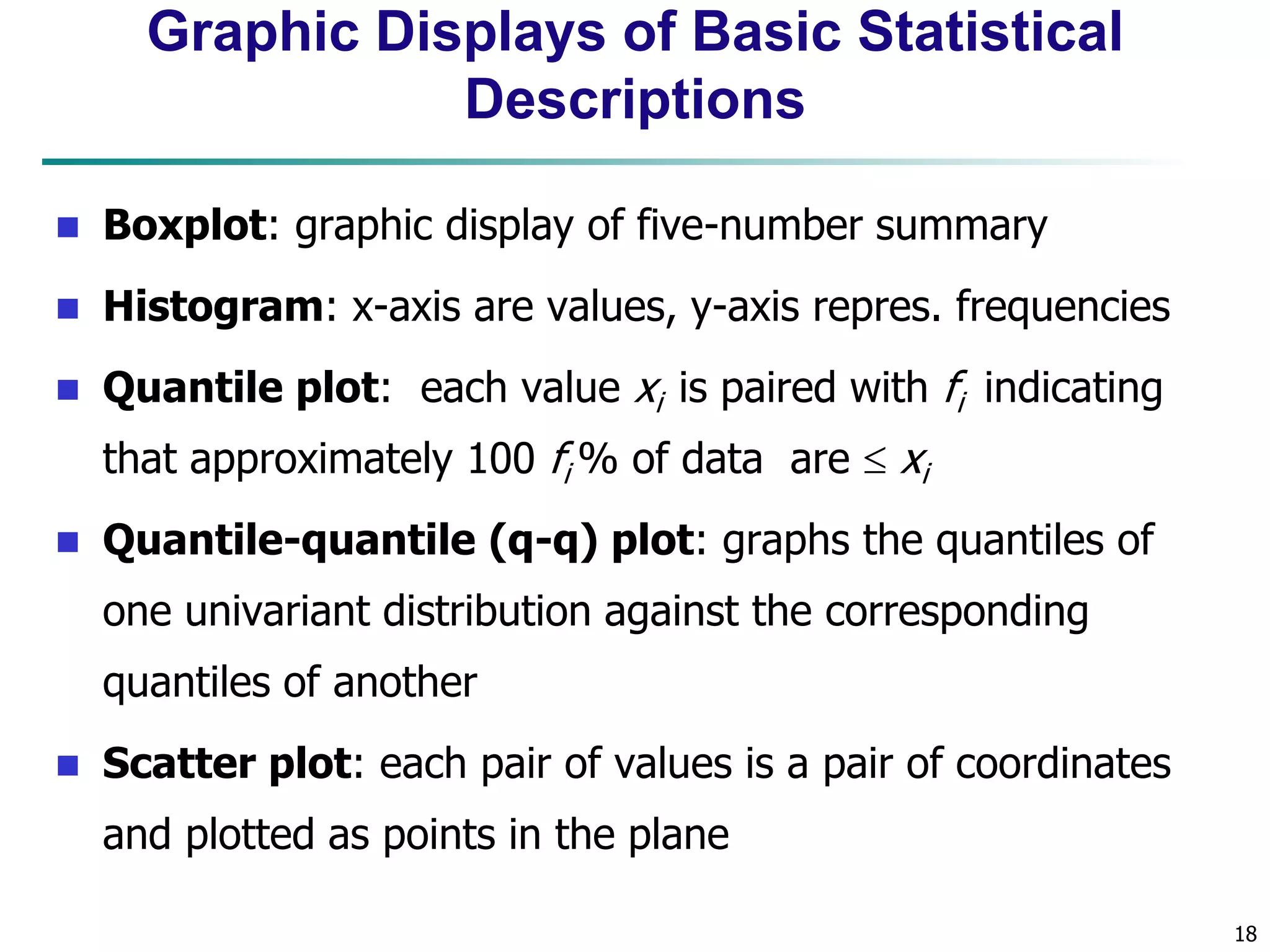
18
Graphic Displays of Basic Statistical
Descriptions
 Boxplot: graphic display of five-number summary
 Histogram: x-axis are values, y-axis repres. frequencies
 Quantile plot: each value xi is paired with fi indicating
that approximately 100 fi % of data are  xi
 Quantile-quantile (q-q) plot: graphs the quantiles of
one univariant distribution against the corresponding
quantiles of another
 Scatter plot: each pair of values is a pair of coordinates
and plotted as points in the plane

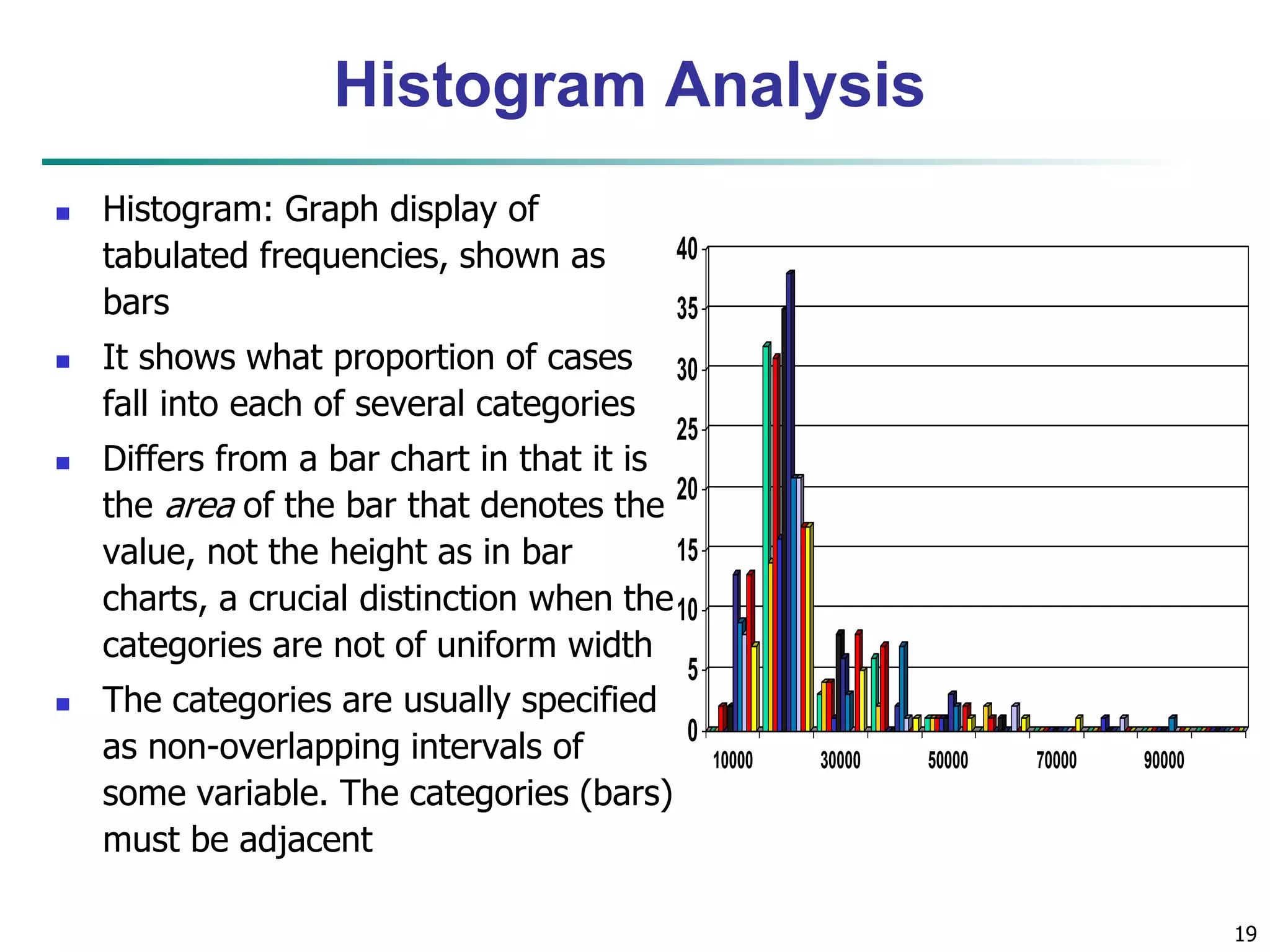
19
Histogram Analysis
 Histogram: Graph display of
tabulated frequencies, shown as
bars
 It shows what proportion of cases
fall into each of several categories
 Differs from a bar chart in that it is
the area of the bar that denotes the
value, not the height as in bar
charts, a crucial distinction when the
categories are not of uniform width
 The categories are usually specified
as non-overlapping intervals of
some variable. The categories (bars)
must be adjacent
40
35
30
25
20
15
10
5
0
10000 30000 50000 70000 90000

20
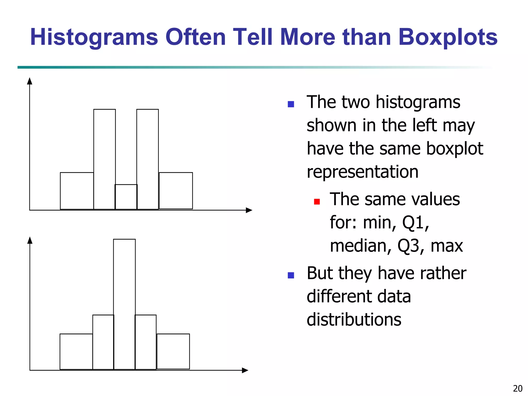
Histograms Often Tell More than Boxplots
 The two histograms
shown in the left may
have the same boxplot
representation
 The same values
for: min, Q1,
median, Q3, max
 But they have rather
different data
distributions

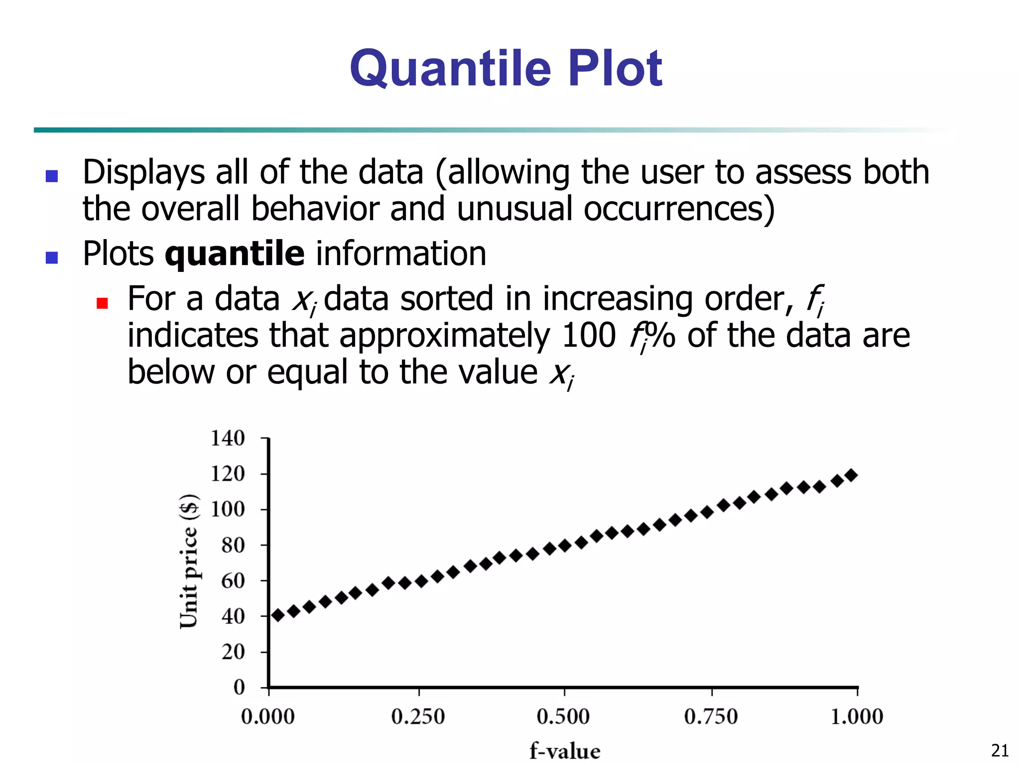
Quantile Plot
 Displays all of the data (allowing the user to assess both
the overall behavior and unusual occurrences)
 Plots quantile information
 For a data xi data sorted in increasing order, fi
indicates that approximately 100 fi% of the data are
below or equal to the value xi
Data Mining: Concepts and Techniques 21

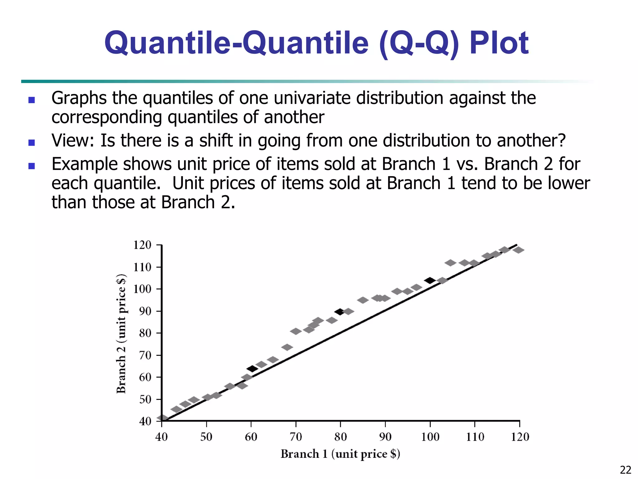
22
Quantile-Quantile (Q-Q) Plot
 Graphs the quantiles of one univariate distribution against the
corresponding quantiles of another
 View: Is there is a shift in going from one distribution to another?
 Example shows unit price of items sold at Branch 1 vs. Branch 2 for
each quantile. Unit prices of items sold at Branch 1 tend to be lower
than those at Branch 2.

23
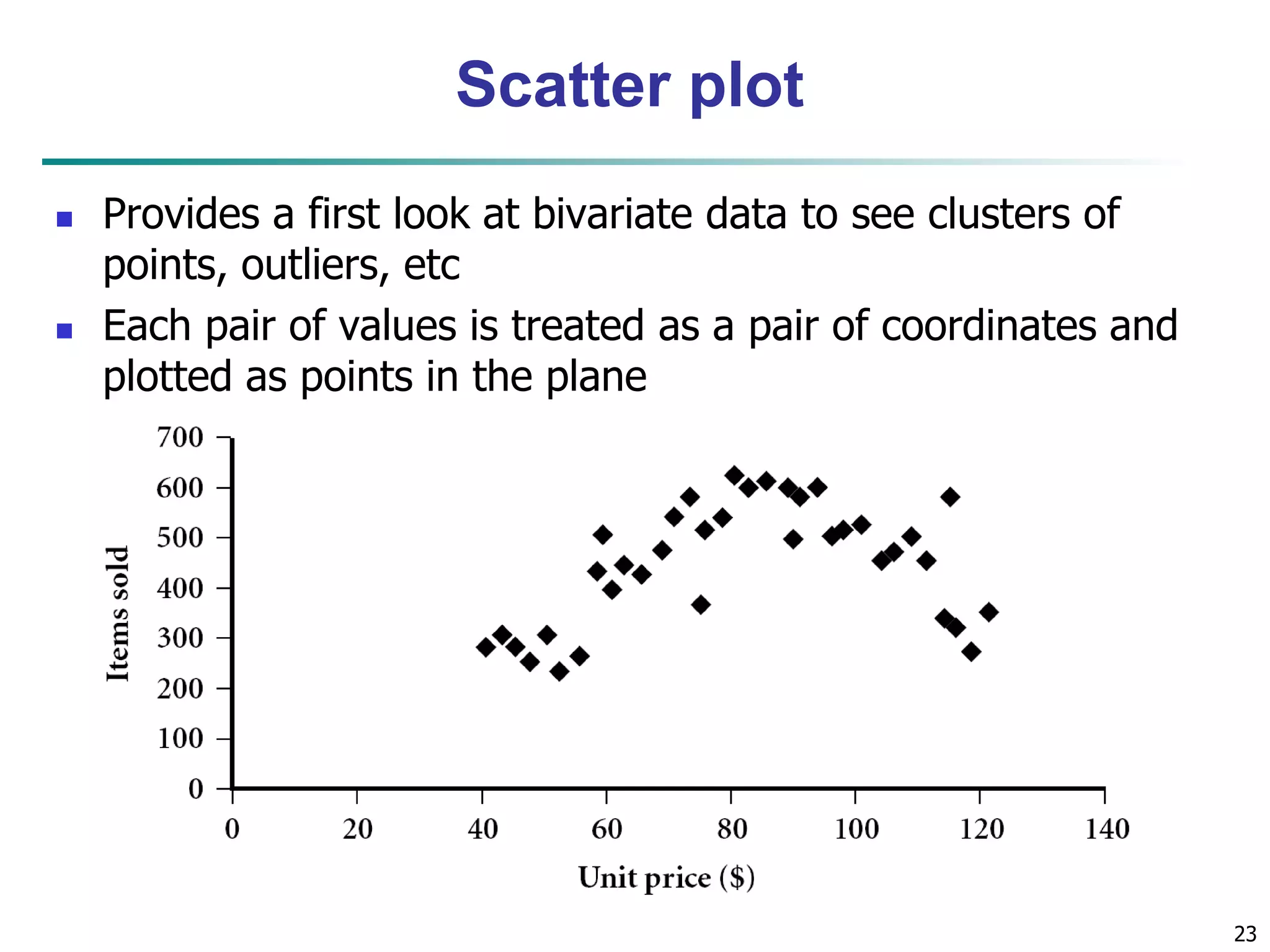
Scatter plot
 Provides a first look at bivariate data to see clusters of
points, outliers, etc
 Each pair of values is treated as a pair of coordinates and
plotted as points in the plane

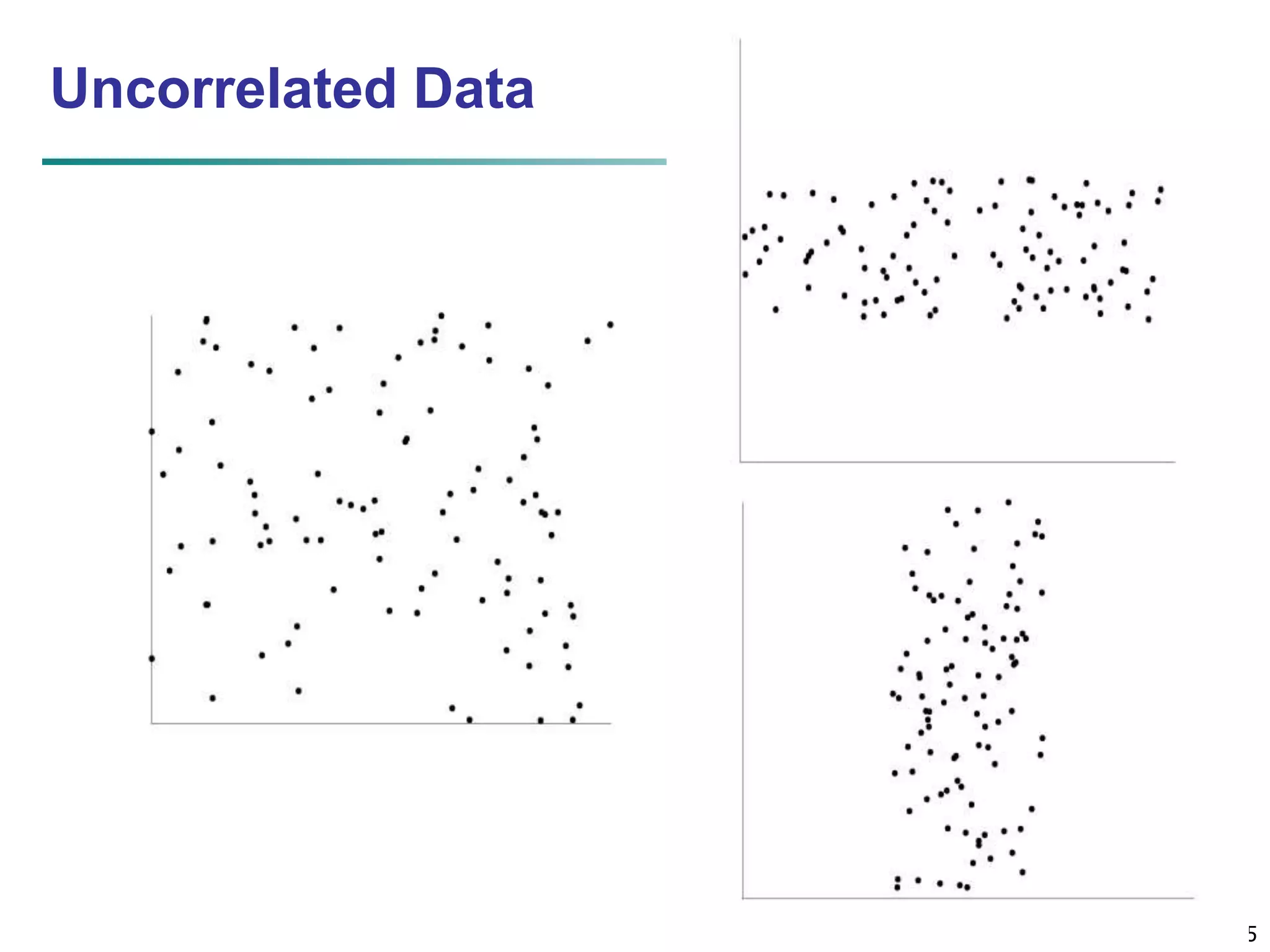
24
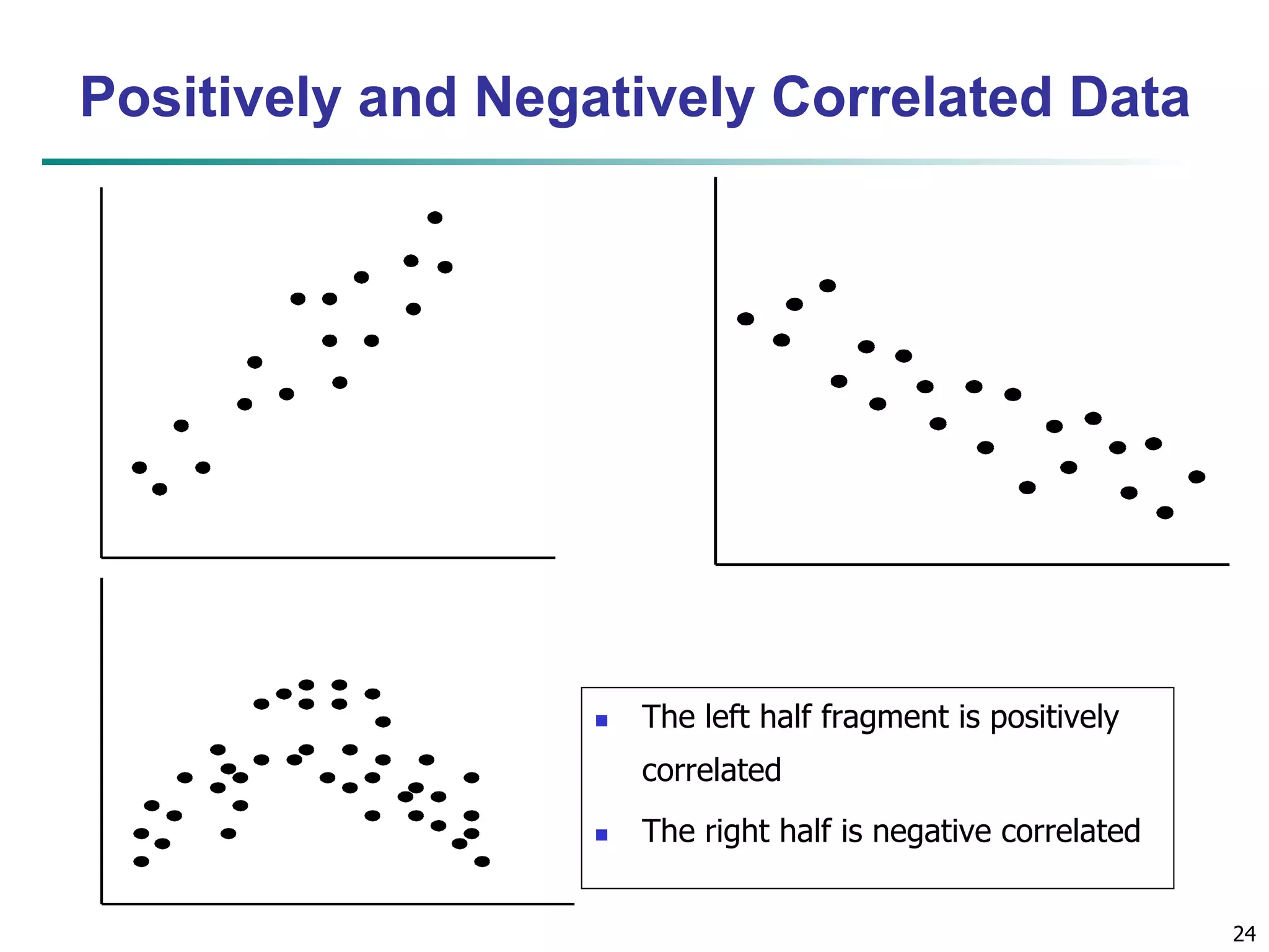
Positively and Negatively Correlated Data
 The left half fragment is positively
correlated
 The right half is negative correlated

26
 Summary

27
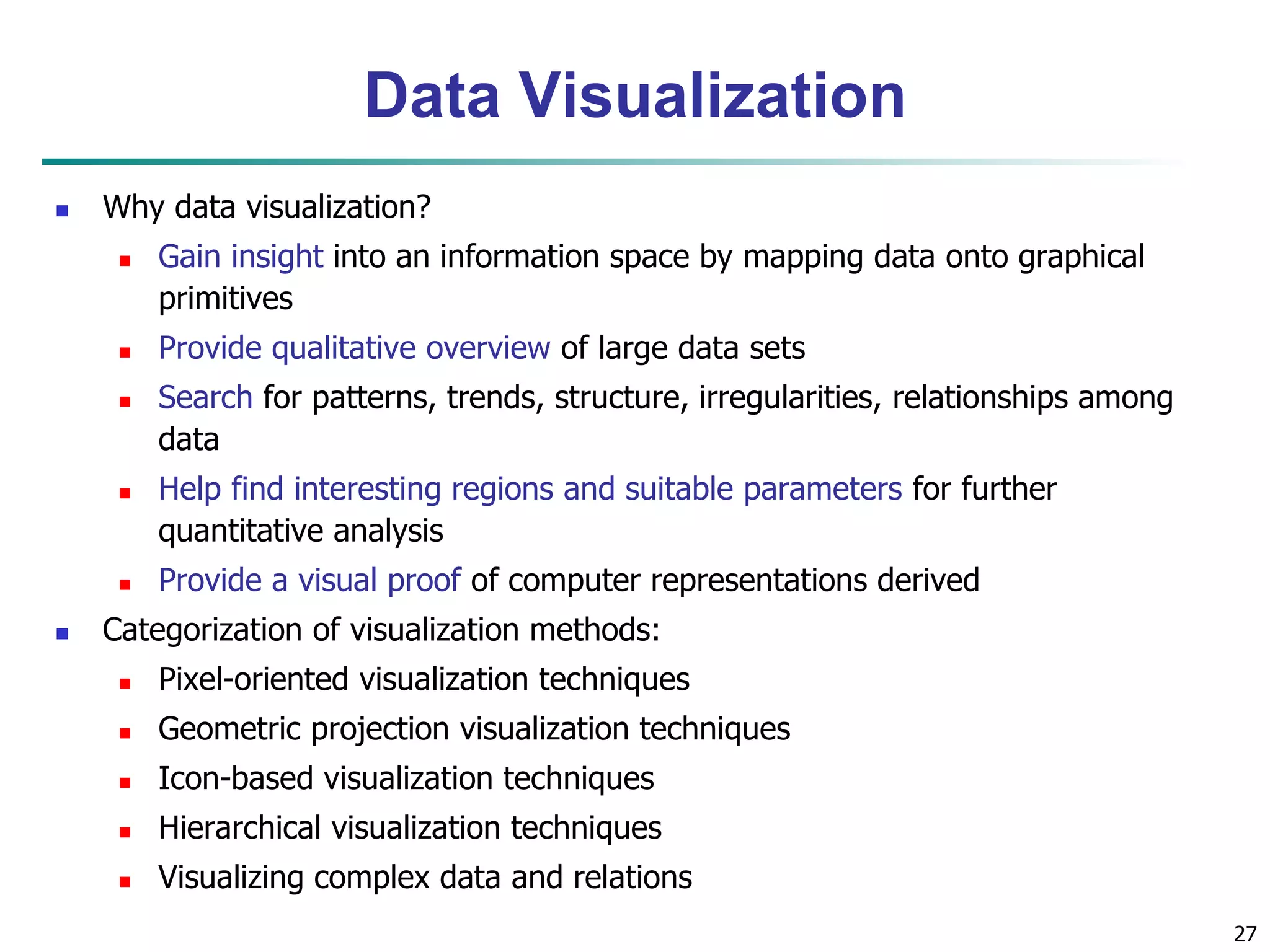
Data Visualization
 Why data visualization?
 Gain insight into an information space by mapping data onto graphical
primitives
 Provide qualitative overview of large data sets
 Search for patterns, trends, structure, irregularities, relationships among
data
 Help find interesting regions and suitable parameters for further
quantitative analysis
 Provide a visual proof of computer representations derived
 Categorization of visualization methods:
 Pixel-oriented visualization techniques
 Geometric projection visualization techniques
 Icon-based visualization techniques
 Hierarchical visualization techniques
 Visualizing complex data and relations

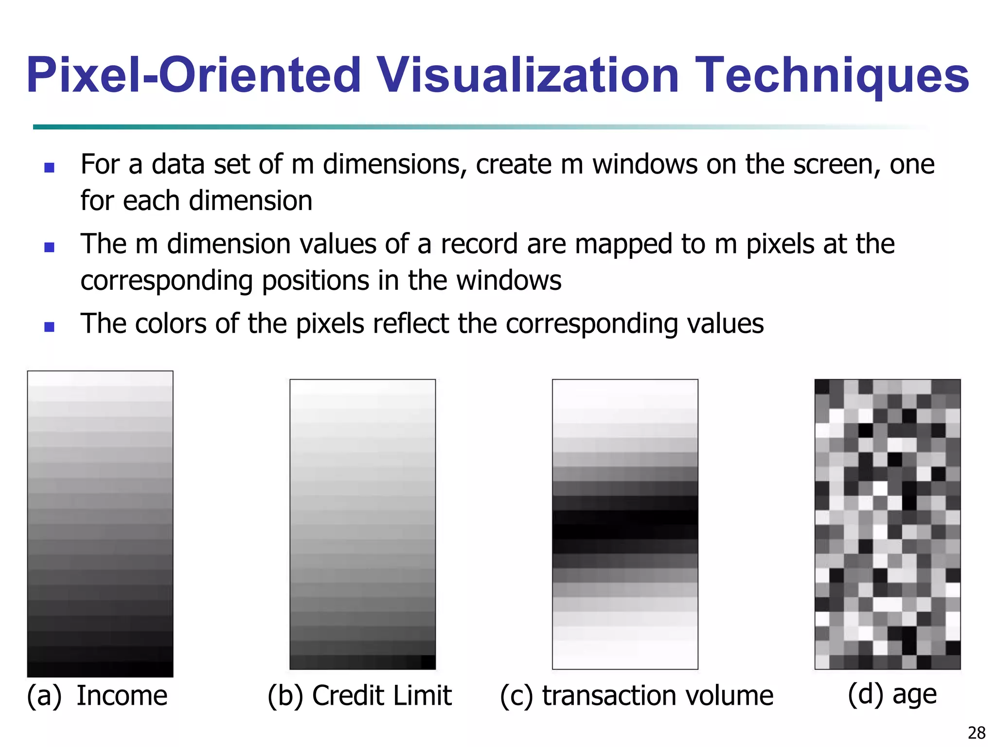
Pixel-Oriented Visualization Techniques
28
 For a data set of m dimensions, create m windows on the screen, one
for each dimension
 The m dimension values of a record are mapped to m pixels at the
corresponding positions in the windows
 The colors of the pixels reflect the corresponding values
(a) Income (b) Credit Limit (c) transaction volume (d) age

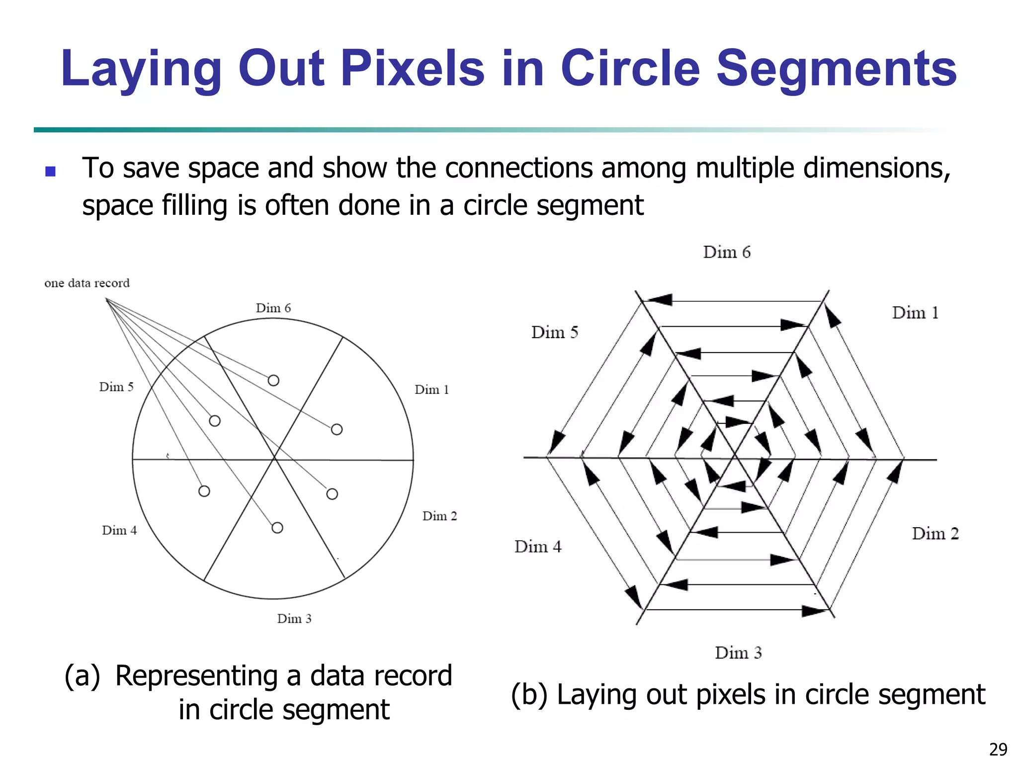
29
Laying Out Pixels in Circle Segments
 To save space and show the connections among multiple dimensions,
space filling is often done in a circle segment
(a) Representing a data record
in circle segment
(b) Laying out pixels in circle segment

30
Geometric Projection Visualization
Techniques
 Visualization of geometric transformations and projections
of the data
 Methods
 Direct visualization
 Scatterplot and scatterplot matrices
 Landscapes
 Projection pursuit technique: Help users find meaningful
projections of multidimensional data
 Prosection views
 Hyperslice
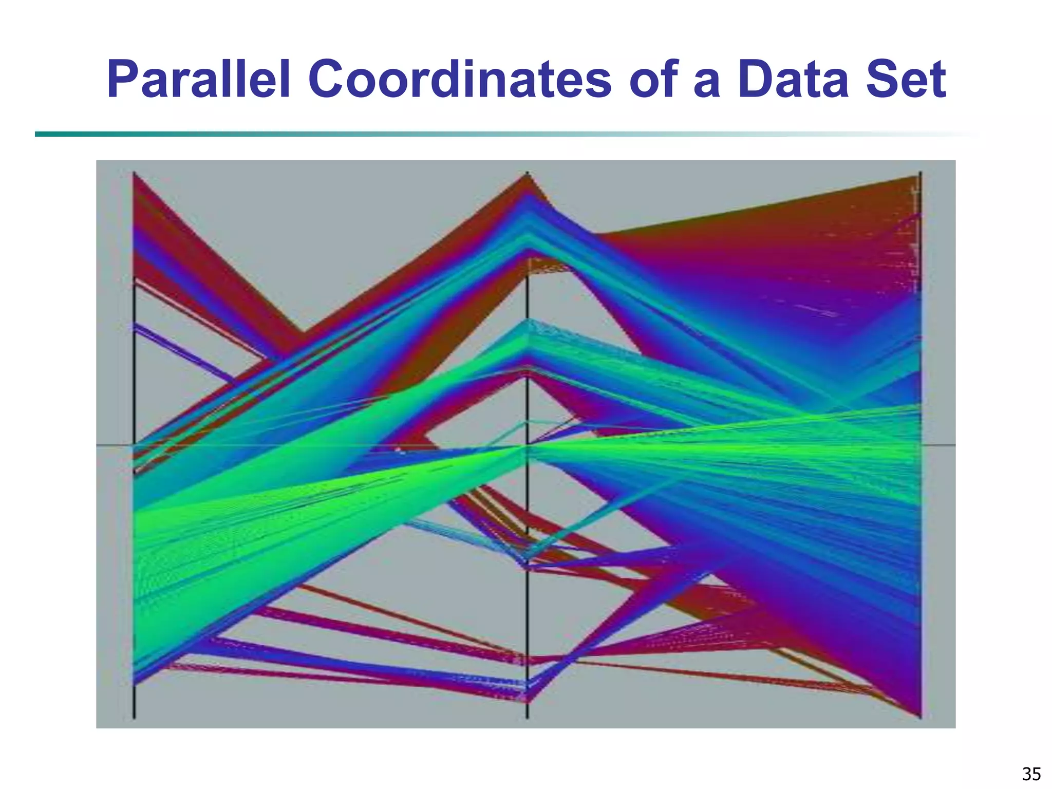
 Parallel coordinates

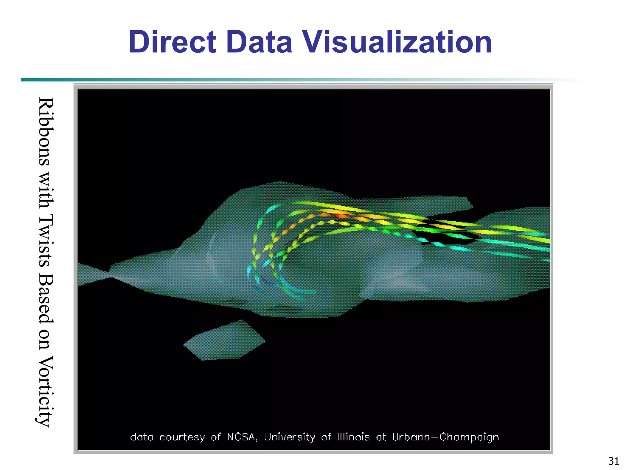
31
Direct Data Visualization
Ribbons with Twists Based on Vorticity

32
Scatterplot Matrices
Used by ermission of M. Ward, Worcester Polytechnic Institute
Matrix of scatterplots (x-y-diagrams) of the k-dim. data [total of (k2/2-k) scatterplots]

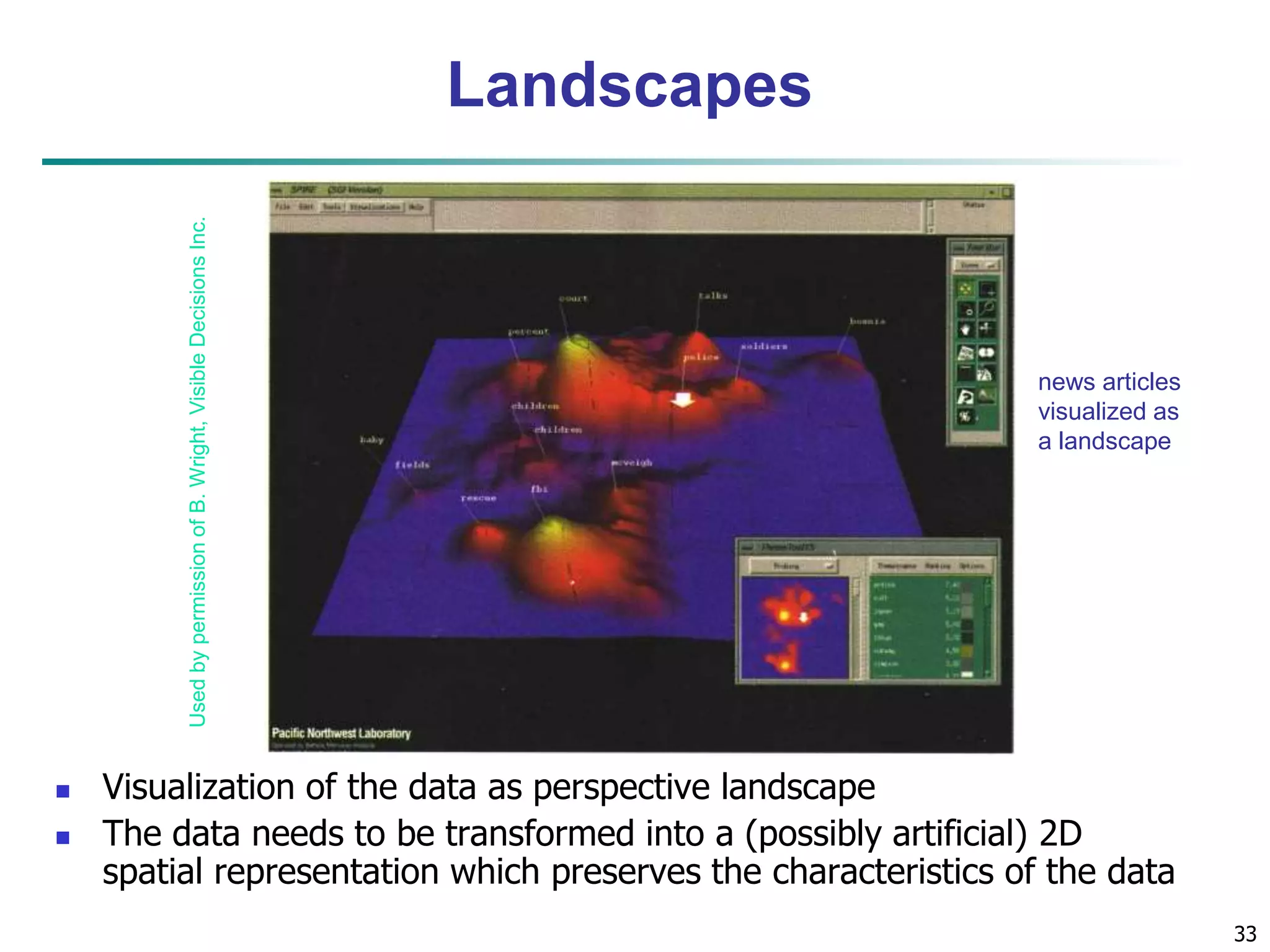
33
news articles
visualized as
a landscape
Used by permission of B. Wright, Visible Decisions Inc.
Landscapes
 Visualization of the data as perspective landscape
 The data needs to be transformed into a (possibly artificial) 2D
spatial representation which preserves the characteristics of the data

34
Parallel Coordinates
 n equidistant axes which are parallel to one of the screen axes and
 The axes are scaled to the [minimum, maximum]: range of the
 Every data item corresponds to a polygonal line which intersects each
of the axes at the point which corresponds to the value for the
attribute
• • •
correspond to the attributes
corresponding attribute
Attr. 1 Attr. 2 Attr. 3 Attr. k

35
Parallel Coordinates of a Data Set

36
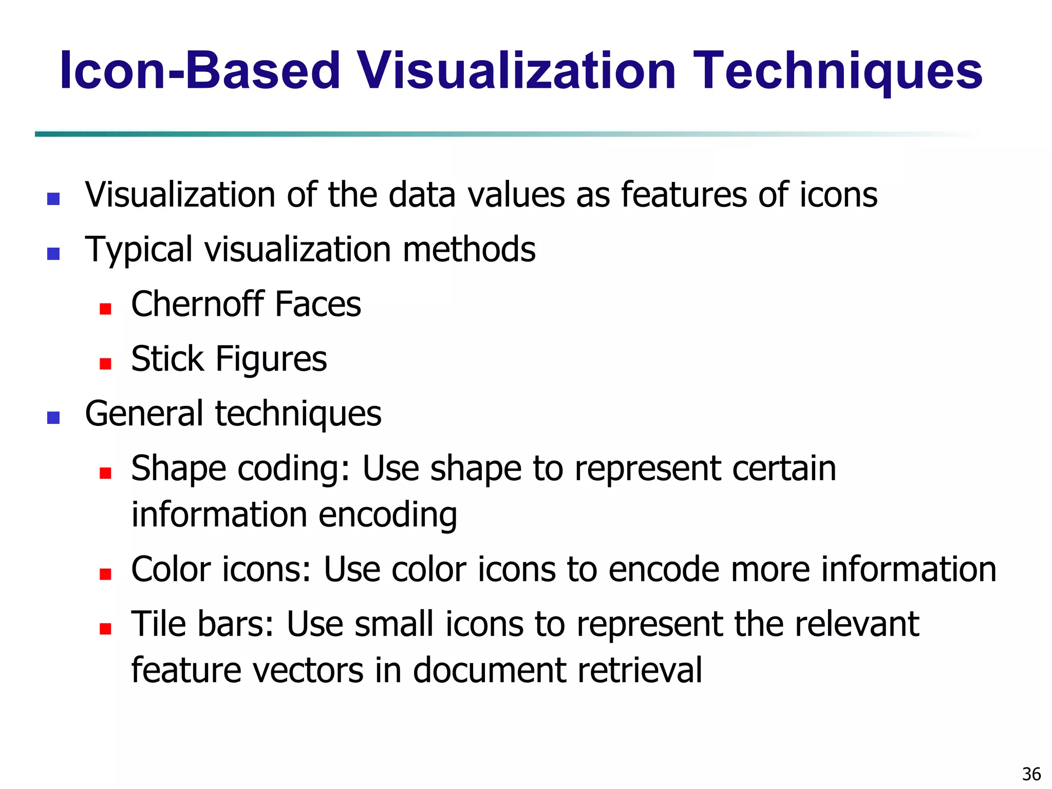
Icon-Based Visualization Techniques
 Visualization of the data values as features of icons
 Typical visualization methods
 Chernoff Faces
 Stick Figures
 General techniques
 Shape coding: Use shape to represent certain
information encoding
 Color icons: Use color icons to encode more information
 Tile bars: Use small icons to represent the relevant
feature vectors in document retrieval

37
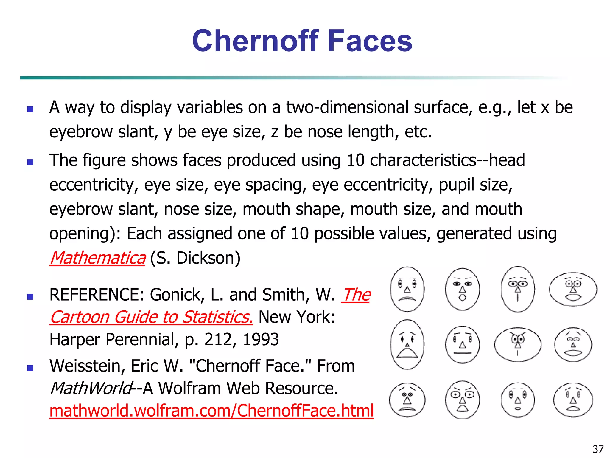
Chernoff Faces
 A way to display variables on a two-dimensional surface, e.g., let x be
eyebrow slant, y be eye size, z be nose length, etc.
 The figure shows faces produced using 10 characteristics--head
eccentricity, eye size, eye spacing, eye eccentricity, pupil size,
eyebrow slant, nose size, mouth shape, mouth size, and mouth
opening): Each assigned one of 10 possible values, generated using
Mathematica (S. Dickson)
 REFERENCE: Gonick, L. and Smith, W. The
Cartoon Guide to Statistics. New York:
Harper Perennial, p. 212, 1993
 Weisstein, Eric W. "Chernoff Face." From
MathWorld--A Wolfram Web Resource.
mathworld.wolfram.com/ChernoffFace.html

38
A census data
figure showing
age, income,
gender,
education, etc.
Stick Figure
A 5-piece stick
figure (1 body
and 4 limbs w.
different
angle/length)

39
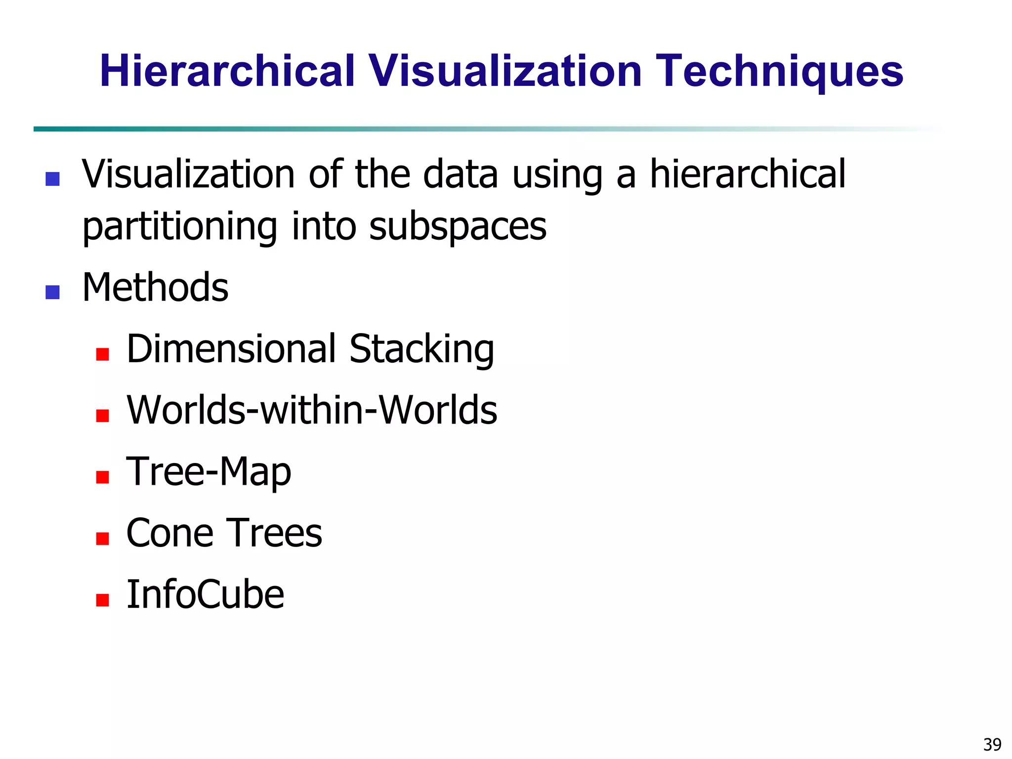
Hierarchical Visualization Techniques
 Visualization of the data using a hierarchical
partitioning into subspaces
 Methods
 Dimensional Stacking
 Worlds-within-Worlds
 Tree-Map
 Cone Trees
 InfoCube

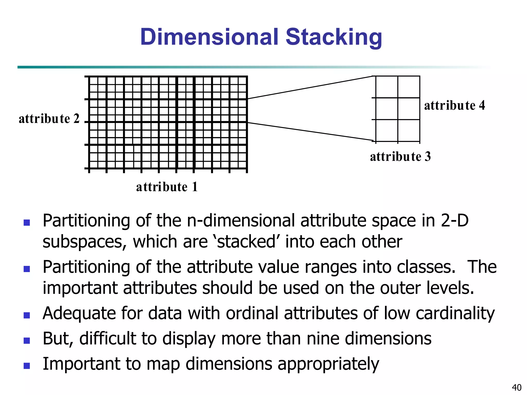
40
Dimensional Stacking
attribute 1
attribute 2
attribute 4
attribute 3
 Partitioning of the n-dimensional attribute space in 2-D
subspaces, which are ‘stacked’ into each other
 Partitioning of the attribute value ranges into classes. The
important attributes should be used on the outer levels.
 Adequate for data with ordinal attributes of low cardinality
 But, difficult to display more than nine dimensions
 Important to map dimensions appropriately

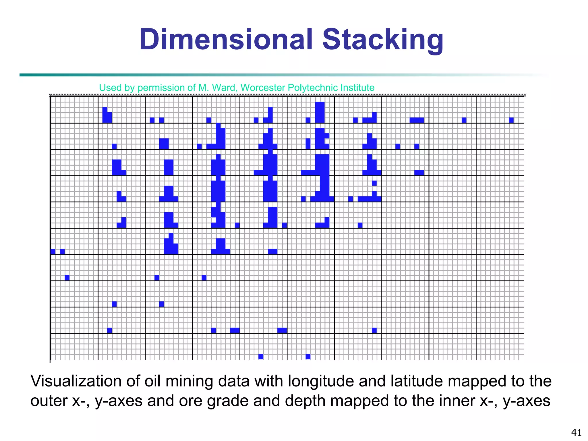
41
Dimensional Stacking
Used by permission of M. Ward, Worcester Polytechnic Institute
Visualization of oil mining data with longitude and latitude mapped to the
outer x-, y-axes and ore grade and depth mapped to the inner x-, y-axes

42
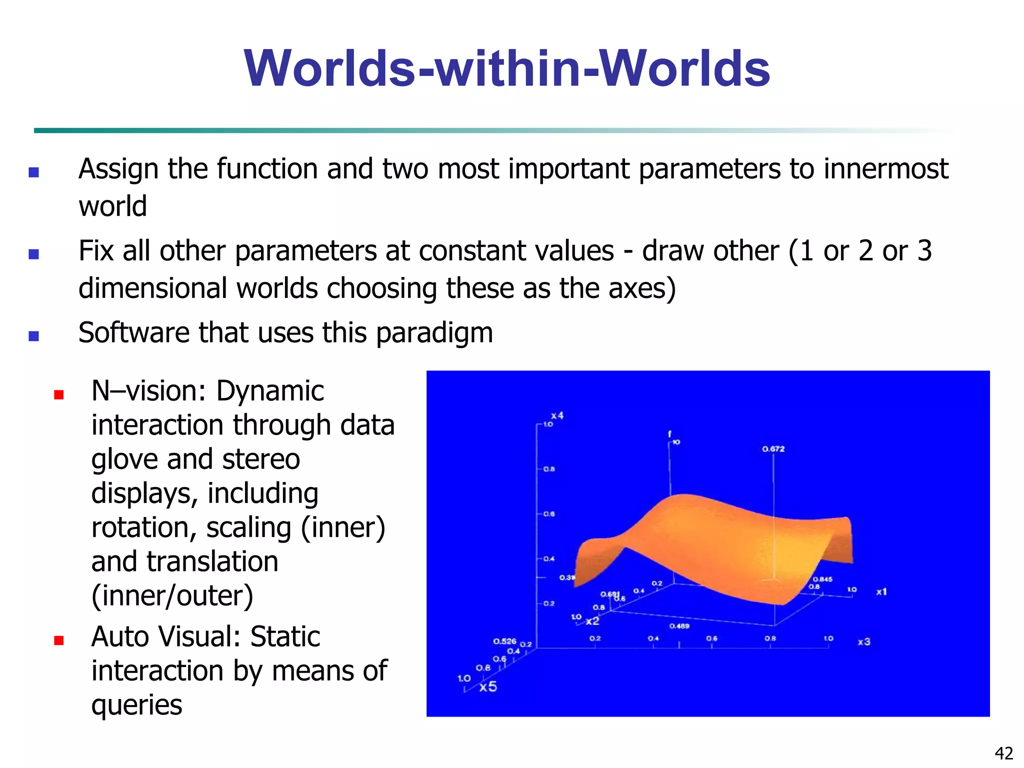
Worlds-within-Worlds
 Assign the function and two most important parameters to innermost
world
 Fix all other parameters at constant values - draw other (1 or 2 or 3
dimensional worlds choosing these as the axes)
 Software that uses this paradigm
 N–vision: Dynamic
interaction through data
glove and stereo
displays, including
rotation, scaling (inner)
and translation
(inner/outer)
 Auto Visual: Static
interaction by means of
queries

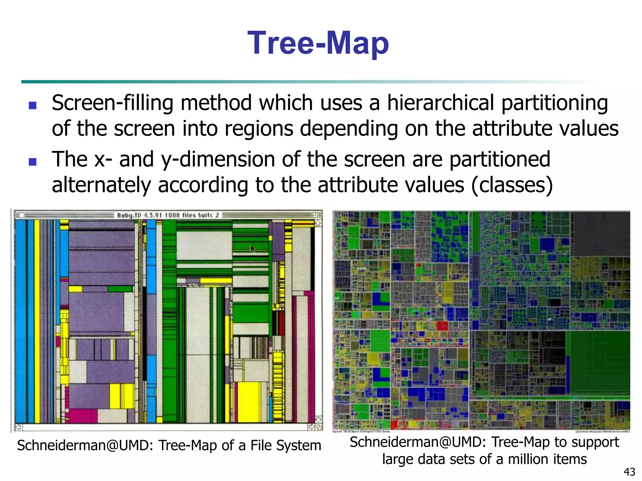
43
Tree-Map
 Screen-filling method which uses a hierarchical partitioning
of the screen into regions depending on the attribute values
 The x- and y-dimension of the screen are partitioned
alternately according to the attribute values (classes)
Schneiderman@UMD: Tree-Map of a File System Schneiderman@UMD: Tree-Map to support
large data sets of a million items

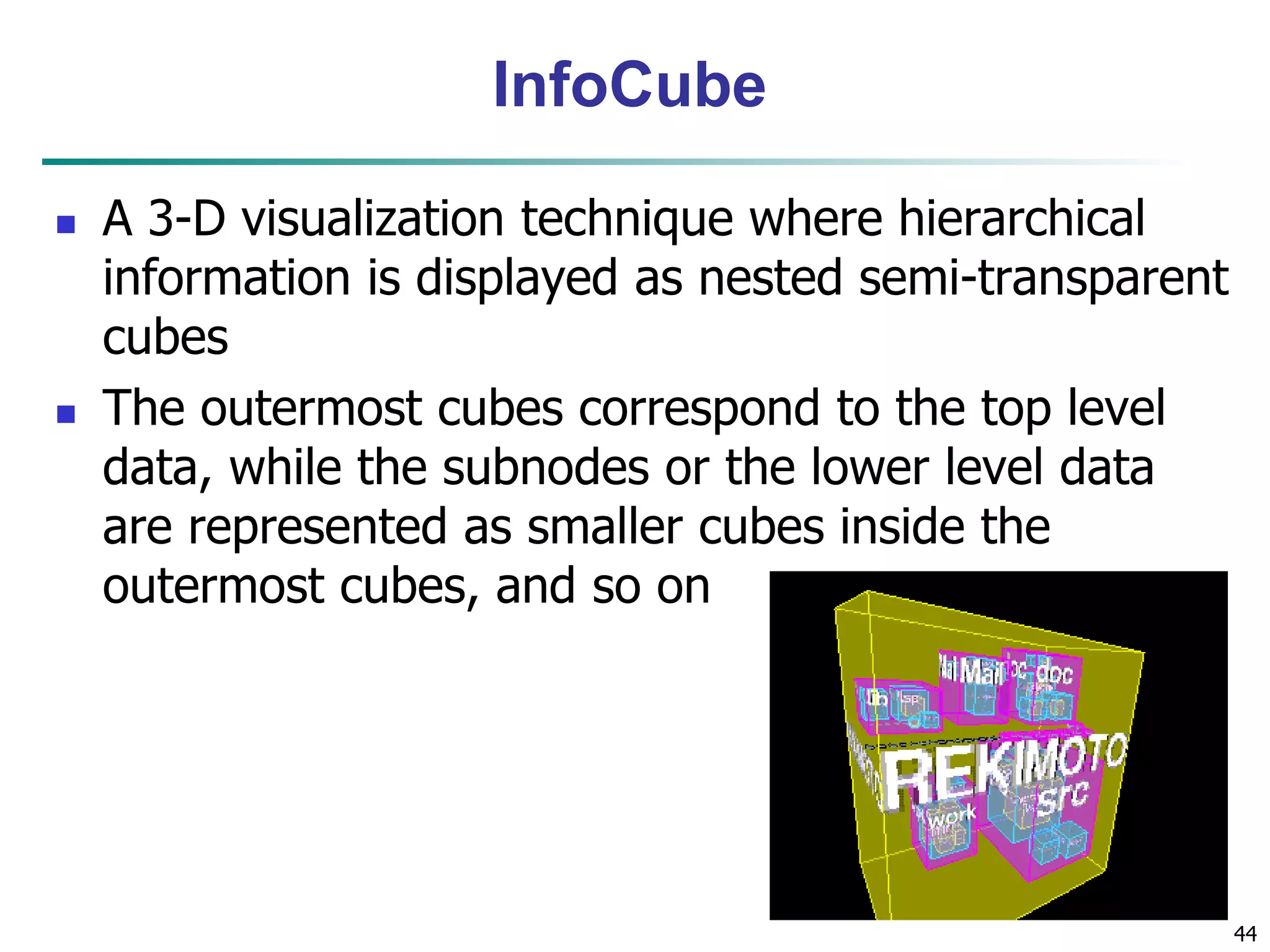
44
InfoCube
 A 3-D visualization technique where hierarchical
information is displayed as nested semi-transparent
cubes
 The outermost cubes correspond to the top level
data, while the subnodes or the lower level data
are represented as smaller cubes inside the
outermost cubes, and so on

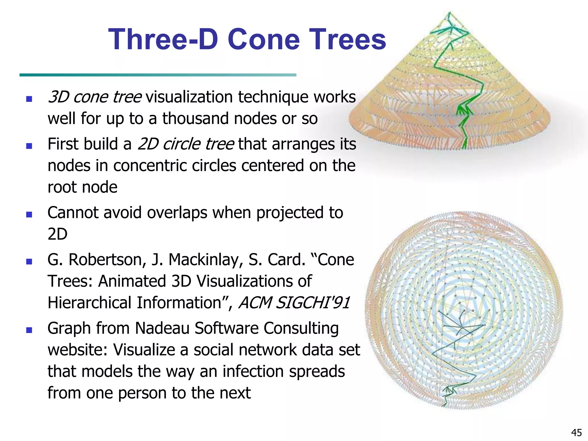
45
Three-D Cone Trees
 3D cone tree visualization technique works
well for up to a thousand nodes or so
 First build a 2D circle tree that arranges its
nodes in concentric circles centered on the
root node
 Cannot avoid overlaps when projected to
2D
 G. Robertson, J. Mackinlay, S. Card. “Cone
Trees: Animated 3D Visualizations of
Hierarchical Information”, ACM SIGCHI'91
 Graph from Nadeau Software Consulting
website: Visualize a social network data set
that models the way an infection spreads
from one person to the next

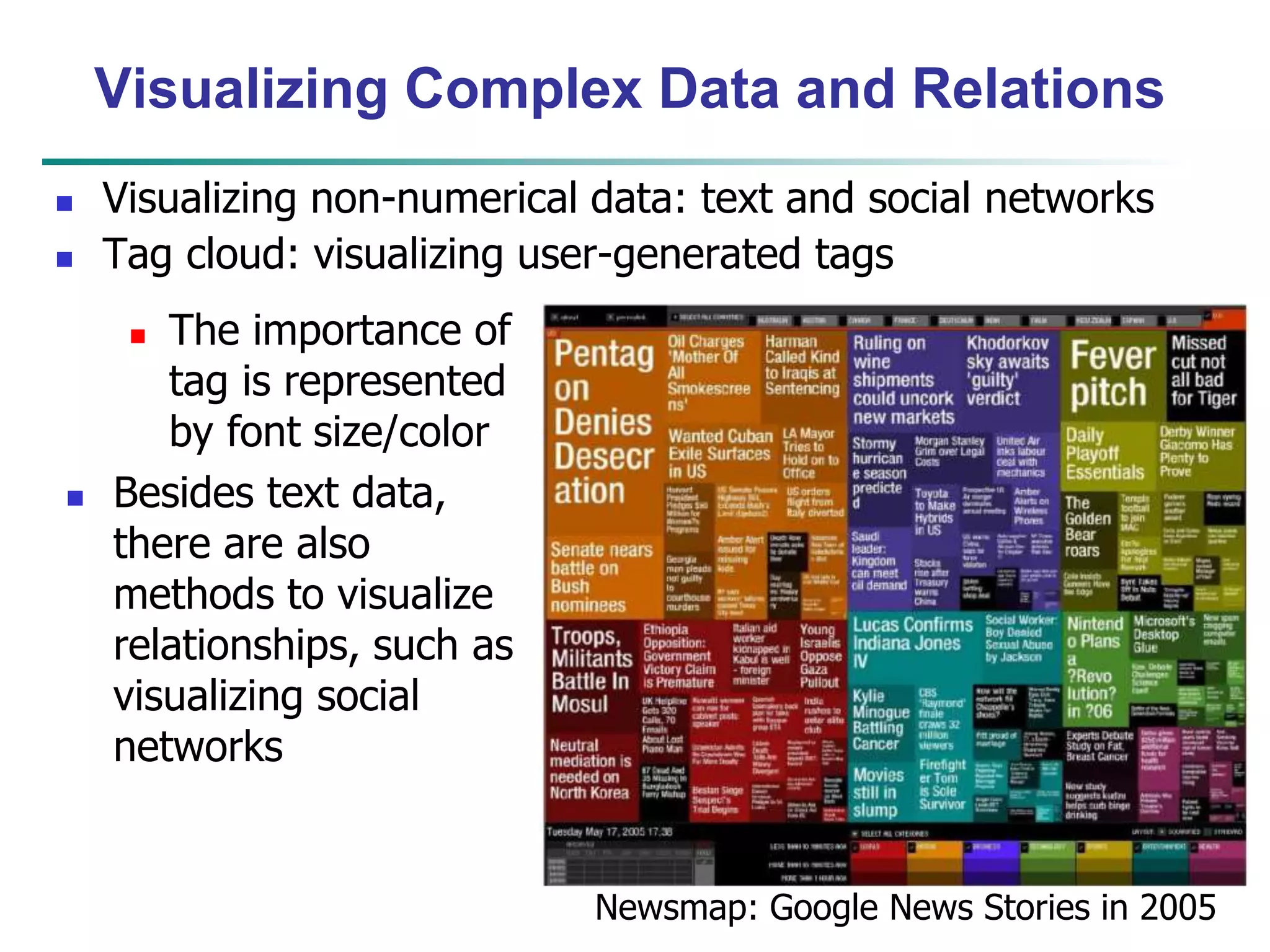
Visualizing Complex Data and Relations
 Visualizing non-numerical data: text and social networks
 Tag cloud: visualizing user-generated tags
 The importance of
tag is represented
by font size/color
 Besides text data,
there are also
methods to visualize
relationships, such as
visualizing social
networks
Newsmap: Google News Stories in 2005

47
 Summary

48
Similarity and Dissimilarity
 Similarity
 Numerical measure of how alike two data objects are
 Value is higher when objects are more alike
 Often falls in the range [0,1]
 Dissimilarity (e.g., distance)
 Numerical measure of how different two data objects
are
 Lower when objects are more alike
 Minimum dissimilarity is often 0
 Upper limit varies
 Proximity refers to a similarity or dissimilarity

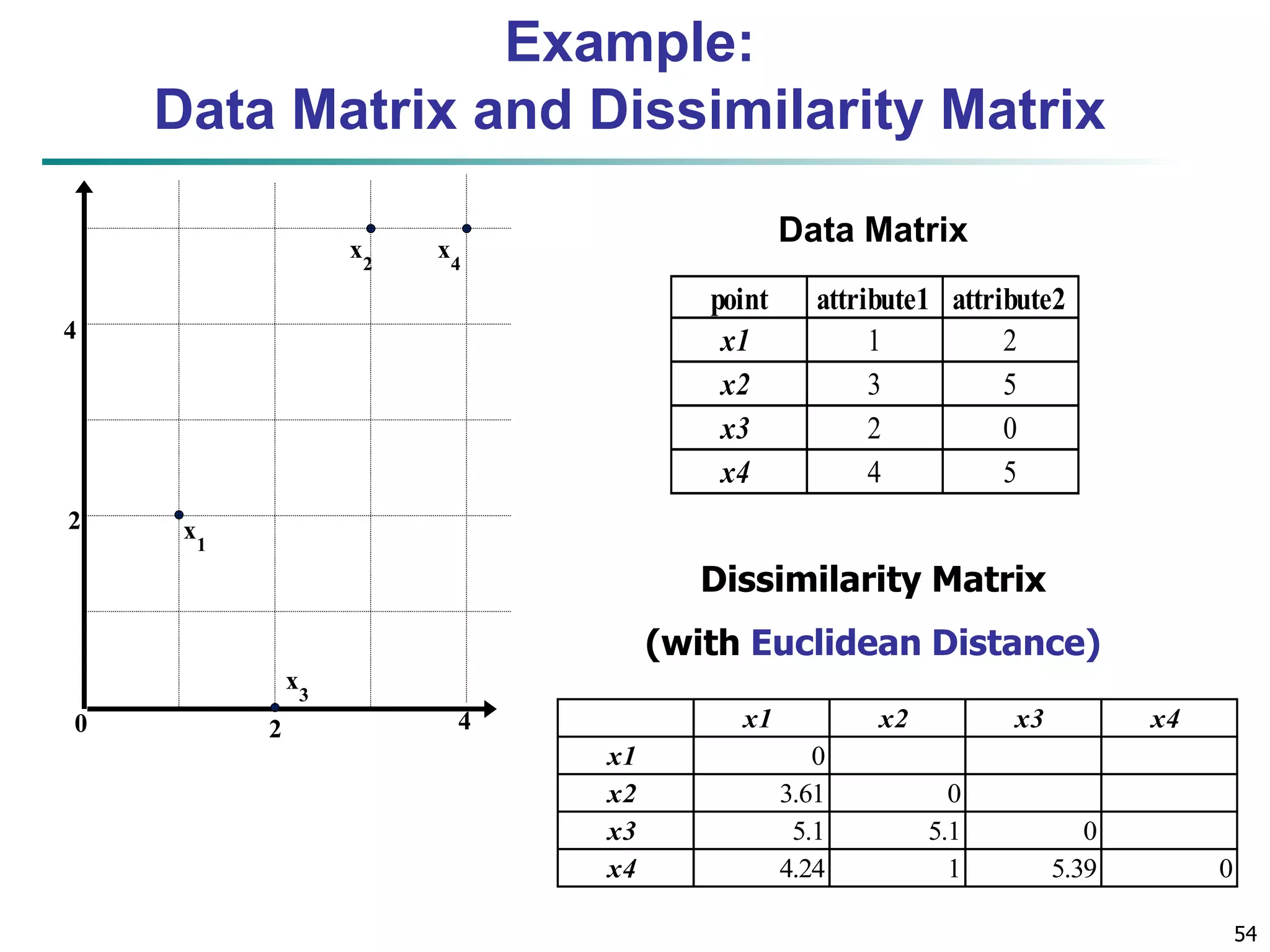
49
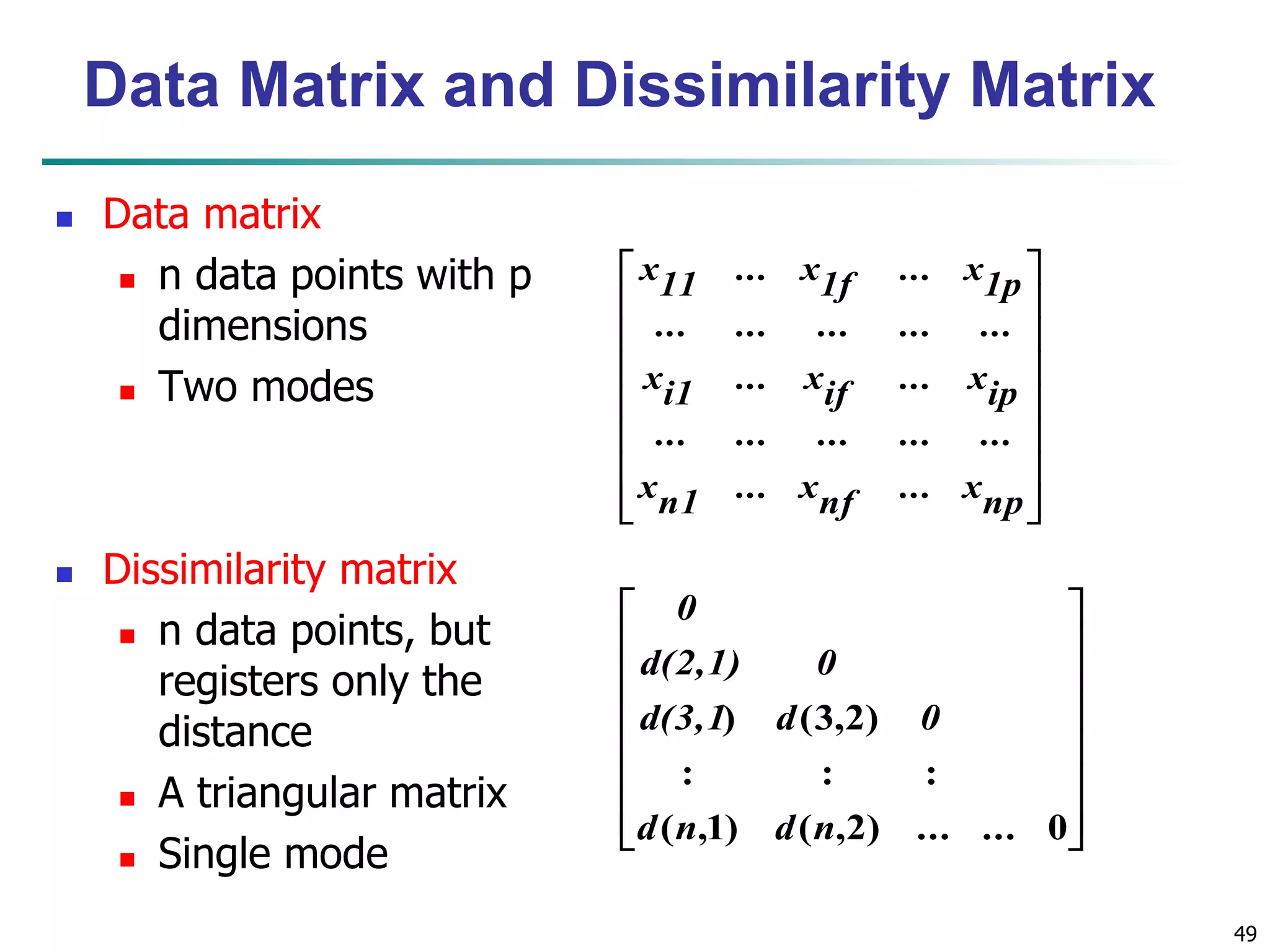
Data Matrix and Dissimilarity Matrix
 Data matrix
 n data points with p
dimensions
 Two modes
 Dissimilarity matrix
 n data points, but
registers only the
distance
 A triangular matrix
 Single mode


















x11 ... x1f ... x1p
... ... ... ... ...
xi1 ... xif ... xip
... ... ... ... ...
np
... x
nf
... x
n1
x
















0
d(2,1) 0
d(3,1 ) d (3,2)
0
: : :
d n d n ...
( ,1) ( ,2) ... 0

50
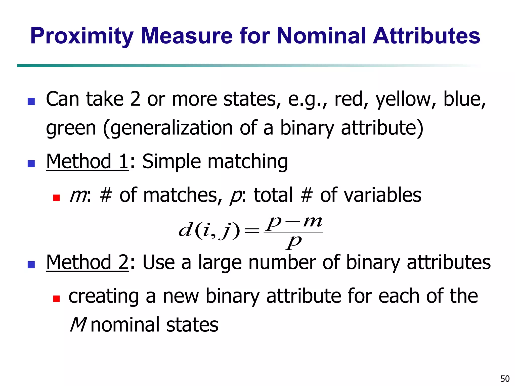
Proximity Measure for Nominal Attributes
 Can take 2 or more states, e.g., red, yellow, blue,
green (generalization of a binary attribute)
 Method 1: Simple matching
 m: # of matches, p: total # of variables
p 
m
p
d i j
( , )
 Method 2: Use a large number of binary attributes
 creating a new binary attribute for each of the
M nominal states

51
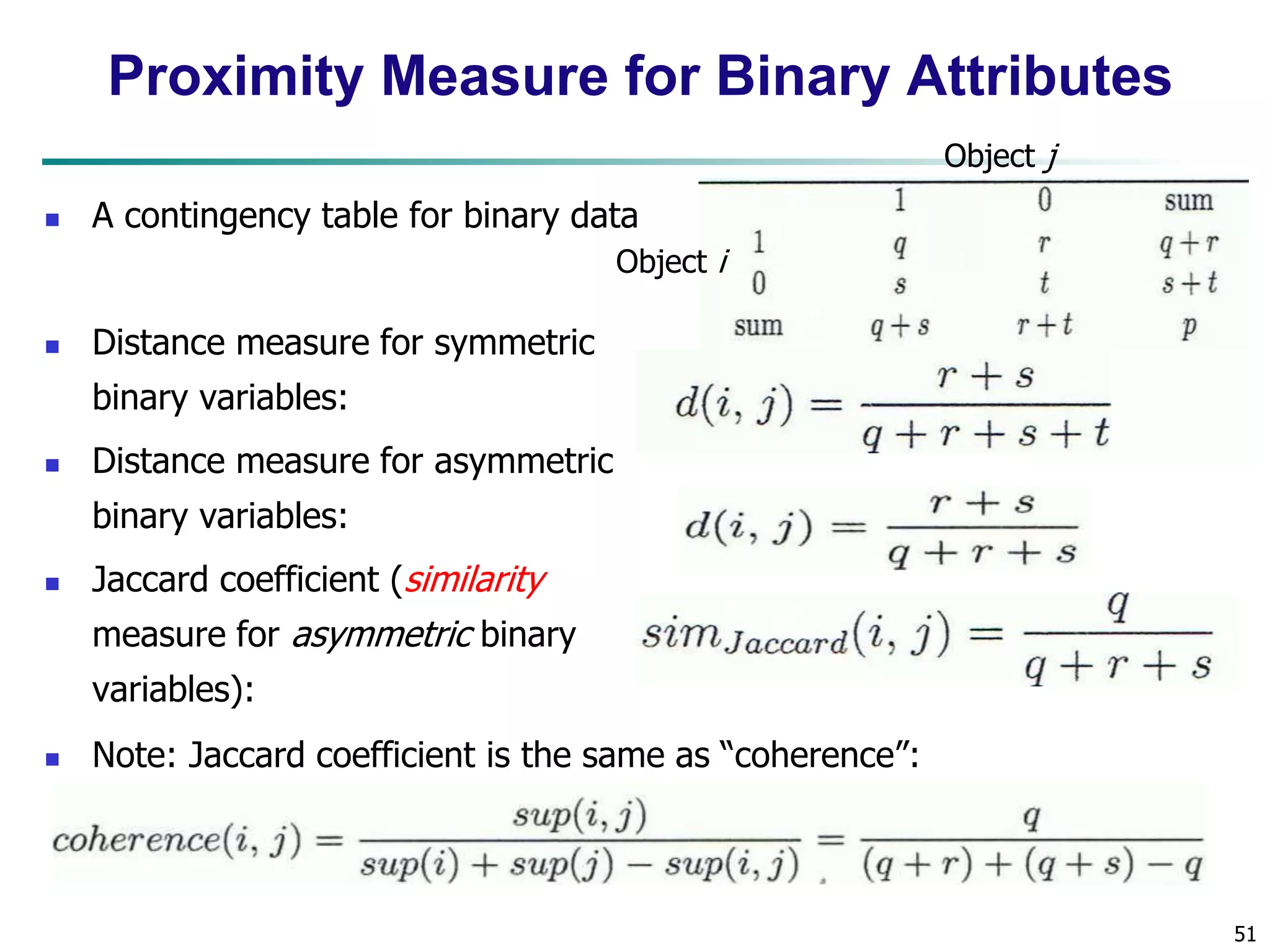
Proximity Measure for Binary Attributes
 A contingency table for binary data
 Distance measure for symmetric
binary variables:
 Distance measure for asymmetric
binary variables:
 Jaccard coefficient (similarity
measure for asymmetric binary
variables):
Object i
 Note: Jaccard coefficient is the same as “coherence”:
Object j

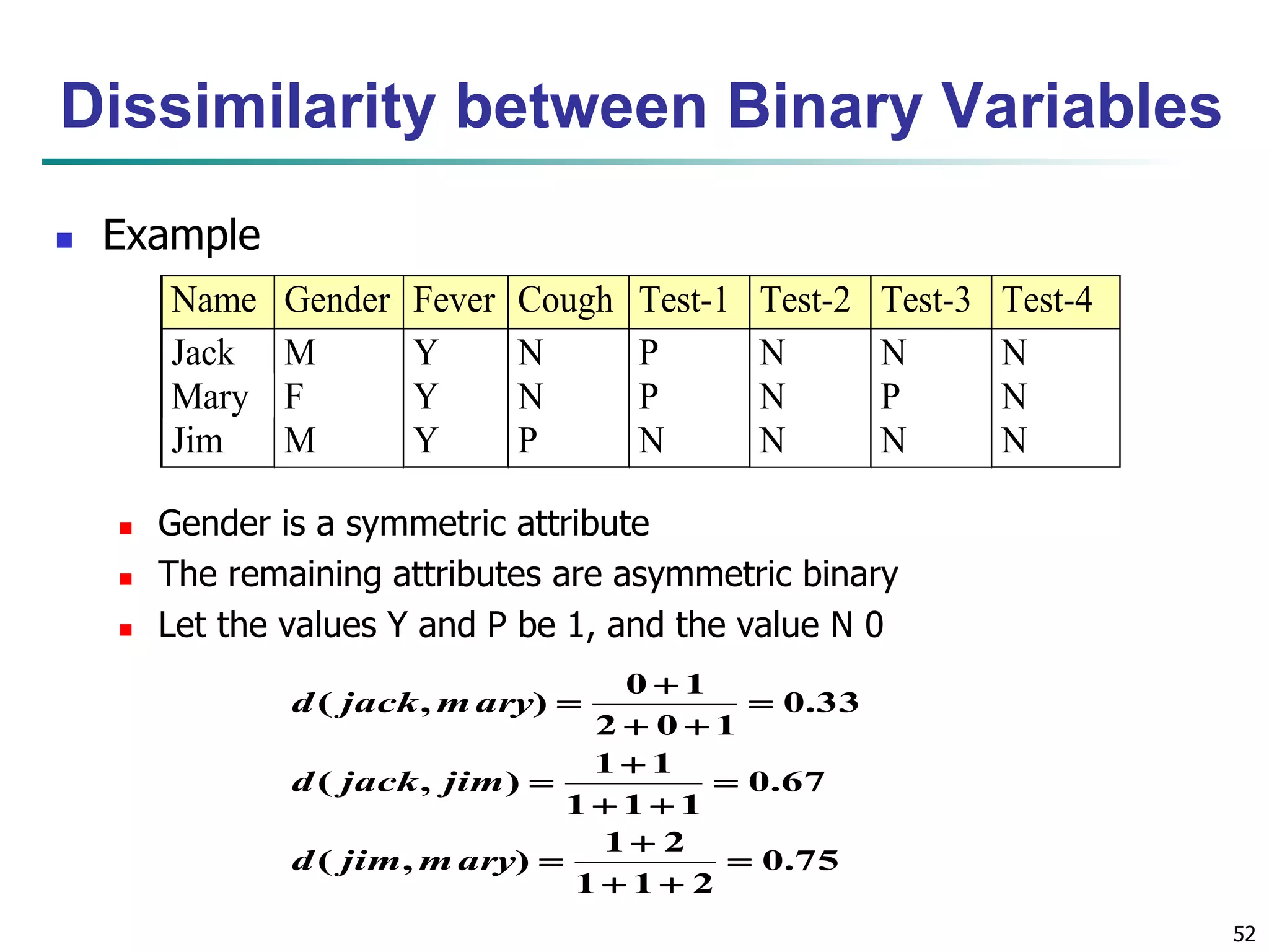
52
Dissimilarity between Binary Variables
 Example
Name Gender Fever Cough Test-1 Test-2 Test-3 Test-4
Jack M Y N P N N N
Mary F Y N P N P N
Jim M Y P N N N N
 Gender is a symmetric attribute
 The remaining attributes are asymmetric binary
 Let the values Y and P be 1, and the value N 0
0.75

0 1

1 1

1 2
1 1 2
d jack mary
d jack jim
( , )
0.67
1 1 1
( , )
0.33
2 0 1
( , )

 


 


 

d jim mary

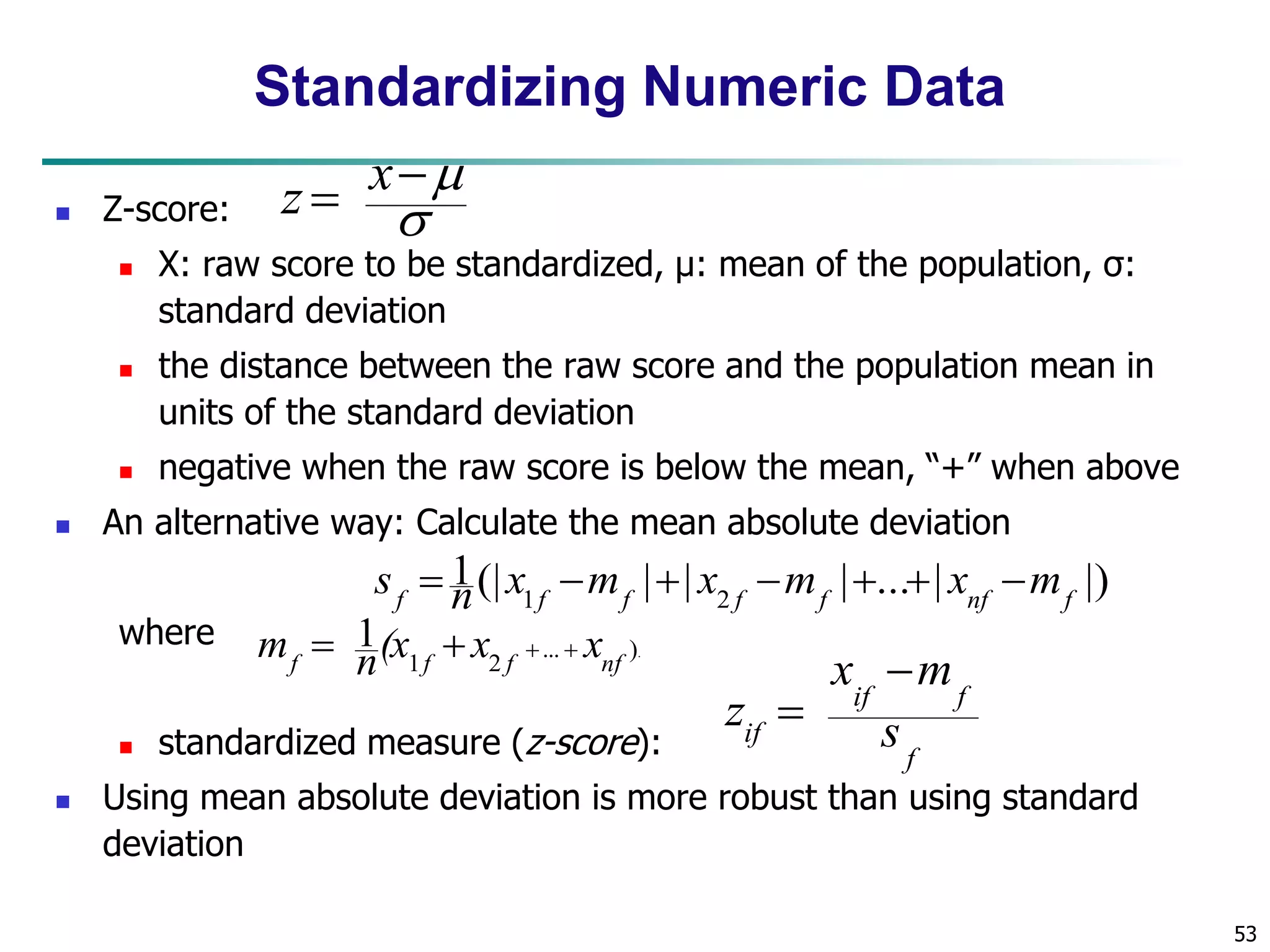
53
Standardizing Numeric Data
 Z-score:

 X: raw score to be standardized, μ: mean of the population, σ:
standard deviation
 the distance between the raw score and the population mean in
units of the standard deviation
 negative when the raw score is below the mean, “+” when above
 An alternative way: Calculate the mean absolute deviation
where
1(| | | | ... | |)
f 1f f 2 f f nf f s  n x m  x m   x m
 standardized measure (z-score):
x 
m
if f
z

 Using mean absolute deviation is more robust than using standard
deviation
... ).
1 2
1
f f f nf m  n(x  x   x
f
if s


x
z

54
Example:
Data Matrix and Dissimilarity Matrix
Data Matrix
point attribute1 attribute2
x1 1 2
x2 3 5
x3 2 0
x4 4 5
Dissimilarity Matrix
(with Euclidean Distance)
x1 x2 x3 x4
x1 0
x2 3.61 0
x3 5.1 5.1 0
x4 4.24 1 5.39 0

55
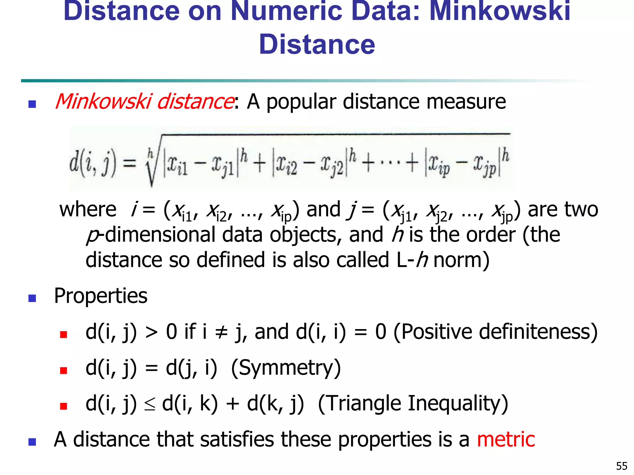
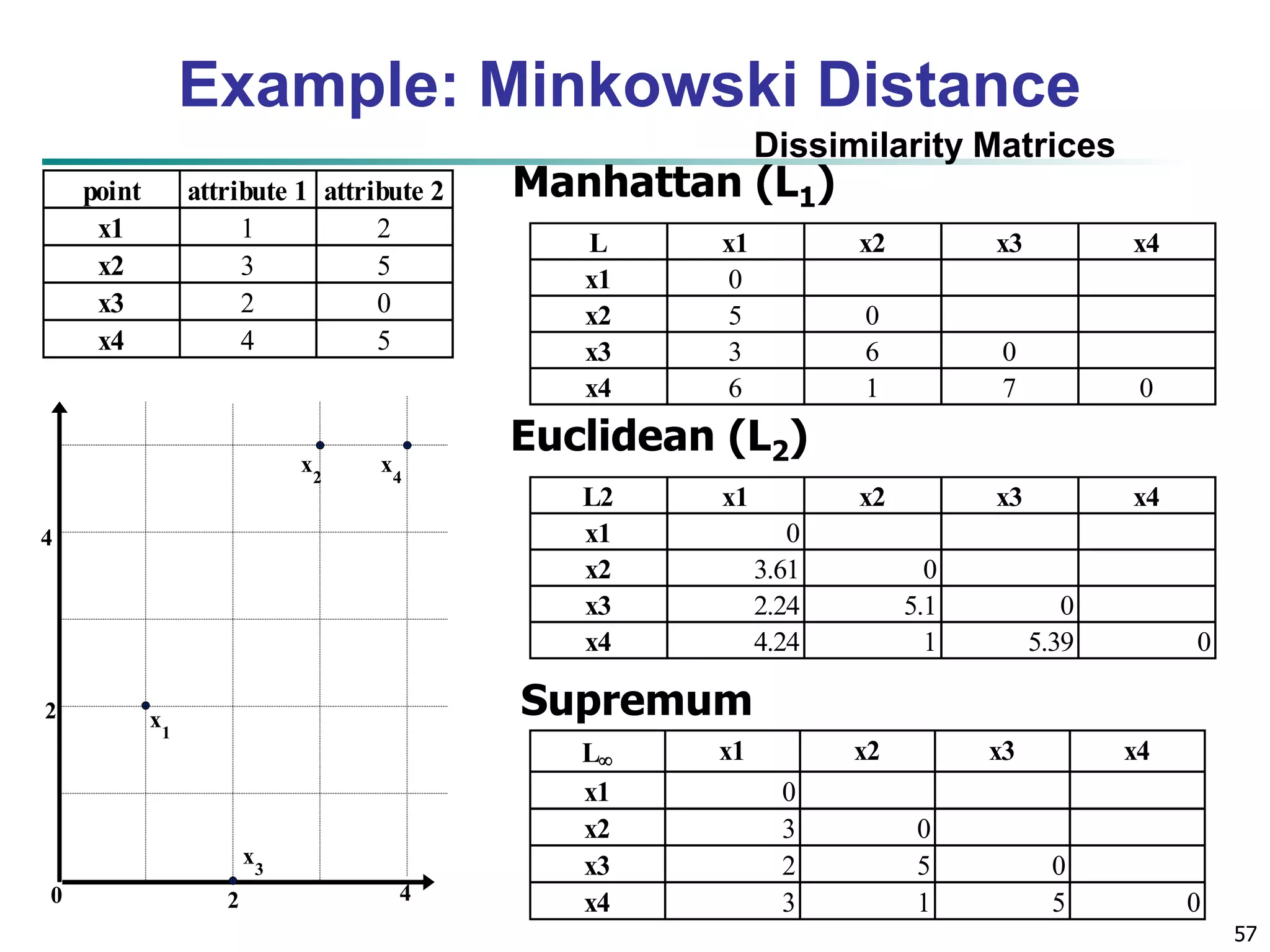
Distance on Numeric Data: Minkowski
Distance
 Minkowski distance: A popular distance measure
where i = (xi1, xi2, …, xip) and j = (xj1, xj2, …, xjp) are two
p-dimensional data objects, and h is the order (the
distance so defined is also called L-h norm)
 Properties
 d(i, j) > 0 if i ≠ j, and d(i, i) = 0 (Positive definiteness)
 d(i, j) = d(j, i) (Symmetry)
 d(i, j)  d(i, k) + d(k, j) (Triangle Inequality)
 A distance that satisfies these properties is a metric

56
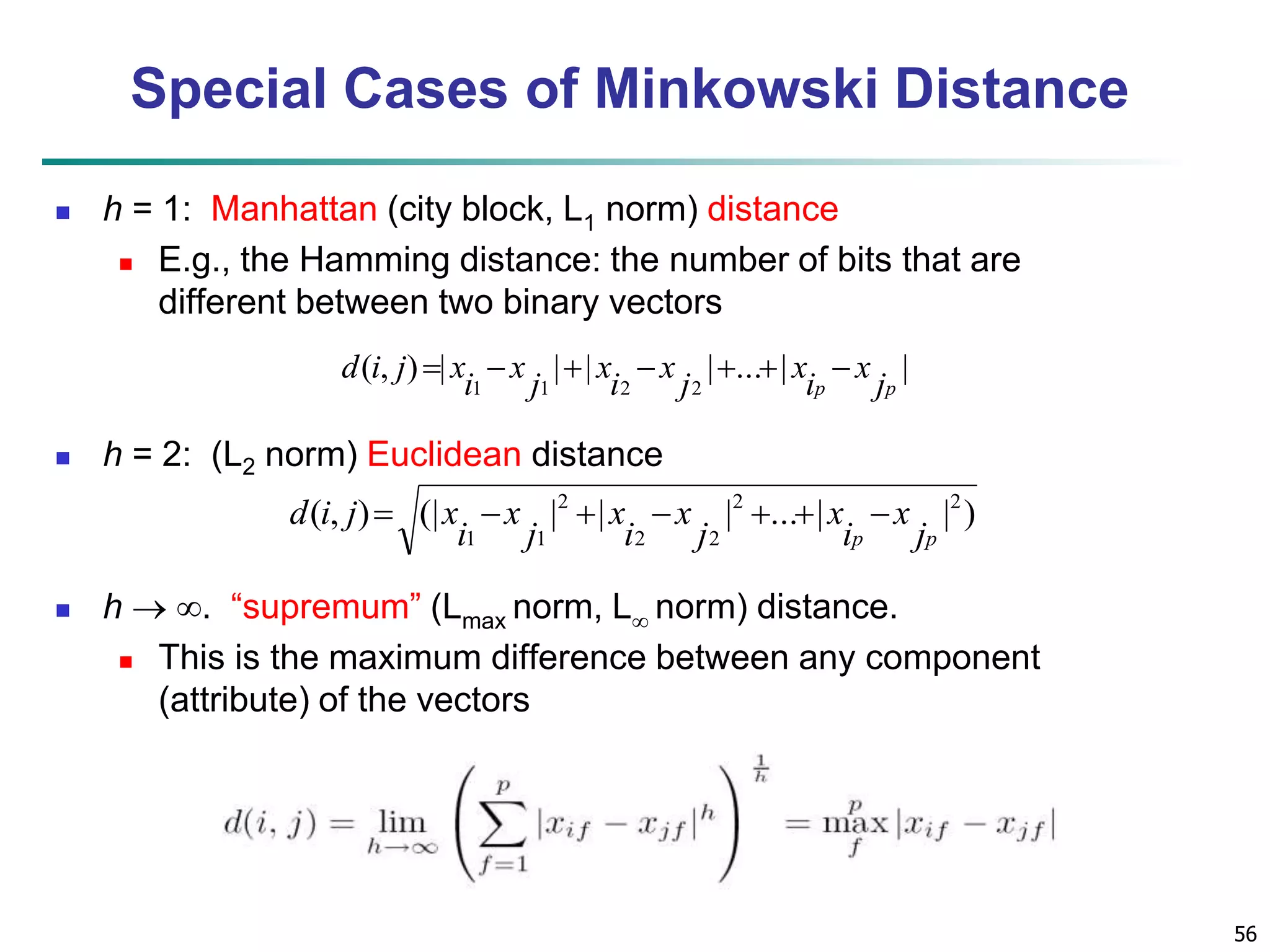
Special Cases of Minkowski Distance
 h = 1: Manhattan (city block, L1 norm) distance
 E.g., the Hamming distance: the number of bits that are
different between two binary vectors
x
d i j  x   x
   x

( , ) | | | | ... | |
 h = 2: (L2 norm) Euclidean distance
( , ) (| | | | 2 ... | x
| 2
) d i j  x   x
   x

 h  . “supremum” (Lmax norm, L norm) distance.
 This is the maximum difference between any component
(attribute) of the vectors
2 2
2
1 1 j
i
p jp
x
i
j
x
i
1 1 2 j
2 i
p jp
x
i
j
x
i

57
Example: Minkowski Distance
Dissimilarity Matrices
point attribute 1 attribute 2
x1 1 2
x2 3 5
x3 2 0
x4 4 5
Manhattan (L1)
L x1 x2 x3 x4
x1 0
x2 5 0
x3 3 6 0
x4 6 1 7 0
Euclidean (L2)
L2 x1 x2 x3 x4
x1 0
x2 3.61 0
x3 2.24 5.1 0
x4 4.24 1 5.39 0
Supremum
L x1 x2 x3 x4
x1 0
x2 3 0
x3 2 5 0
x4 3 1 5 0

58
Ordinal Variables
 An ordinal variable can be discrete or continuous
 Order is important, e.g., rank
 Can be treated like interval-scaled
 replace xif by their rank
 map the range of each variable onto [0, 1] by replacing
i-th object in the f-th variable by
1

r
z
 compute the dissimilarity using methods for interval-scaled
variables
1


f
if
if M
{1,..., } if f r  M

59
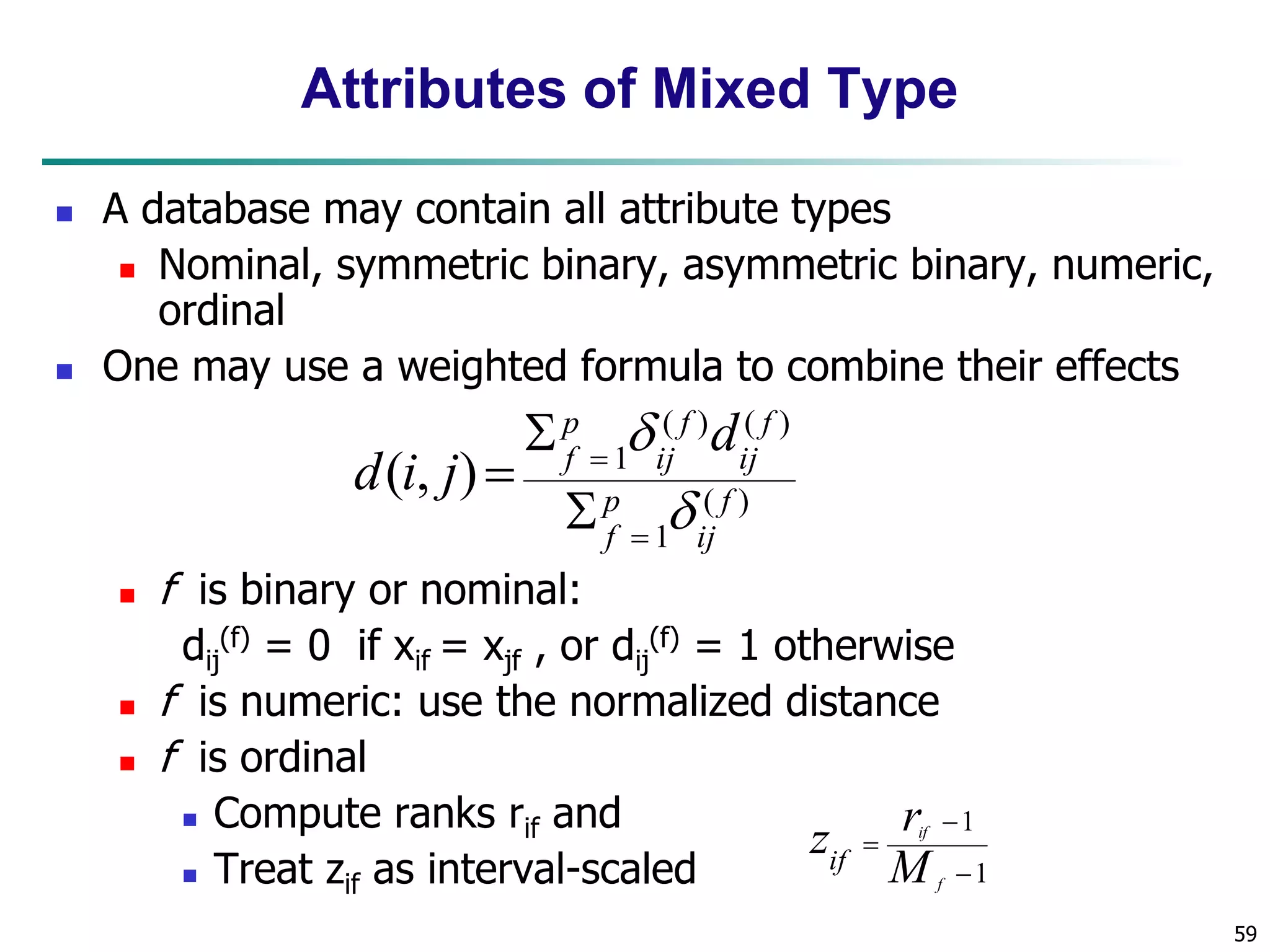
Attributes of Mixed Type
 A database may contain all attribute types
 Nominal, symmetric binary, asymmetric binary, numeric,
ordinal
 One may use a weighted formula to combine their effects
p
f d
 f is binary or nominal:

(f) = 0 if xif = xjf , or dij
dij
( ) ( )
(f) = 1 otherwise
 f is numeric: use the normalized distance
 f is ordinal
 Compute ranks rif and
 Treat zif as interval-scaled
( )
1
1 ( , )
f
ij
p
f
f
ij
f
ij
d i j






1

1


f
r
if
M
zif

60
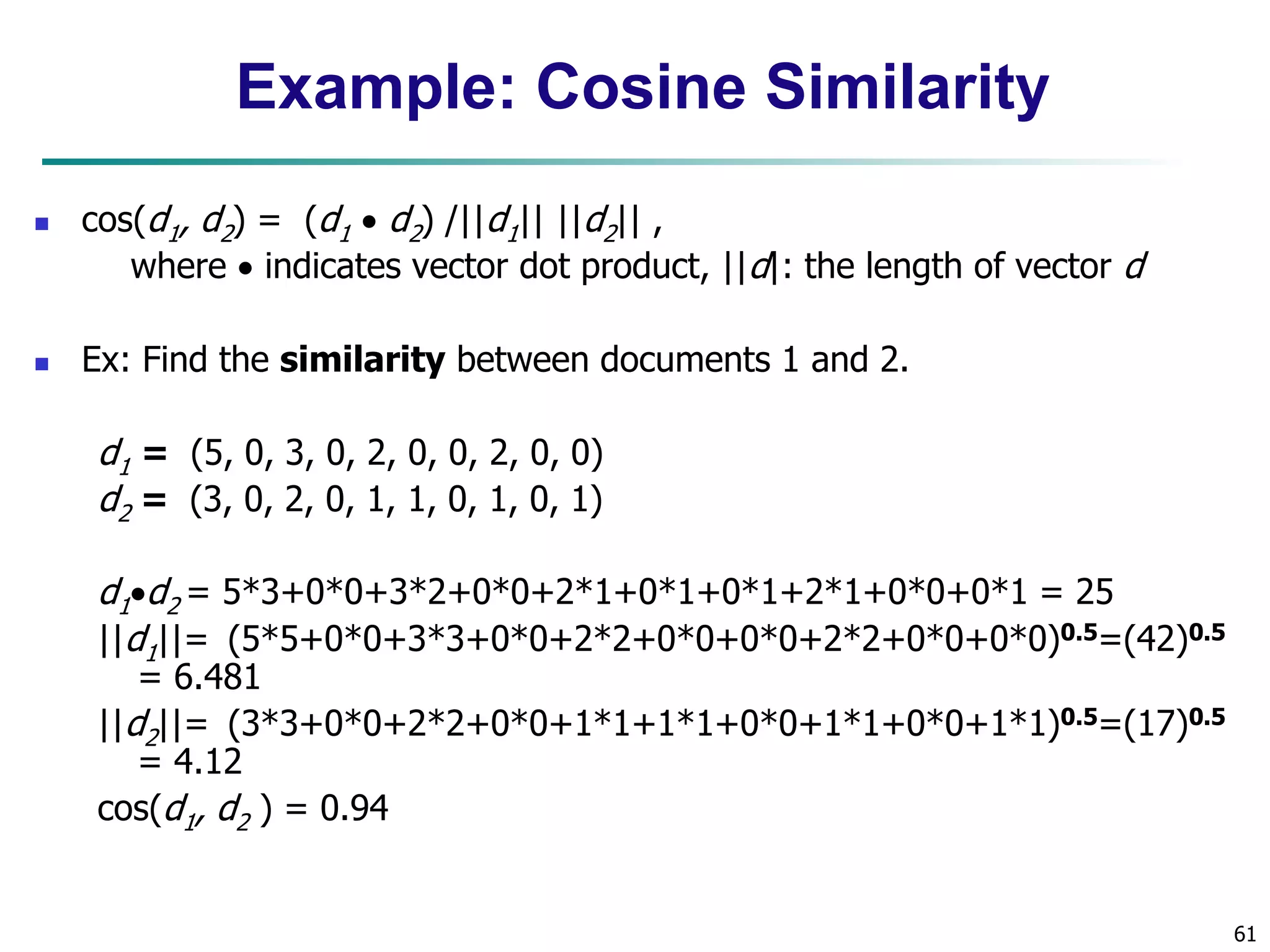
Cosine Similarity
 A document can be represented by thousands of attributes, each
recording the frequency of a particular word (such as keywords) or
phrase in the document.
 Other vector objects: gene features in micro-arrays, …
 Applications: information retrieval, biologic taxonomy, gene feature
mapping, ...
 Cosine measure: If d1 and d2 are two vectors (e.g., term-frequency
vectors), then
cos(d1, d2) = (d1  d2) /||d1|| ||d2|| ,
where  indicates vector dot product, ||d||: the length of vector d

61
Example: Cosine Similarity
 cos(d1, d2) = (d1  d2) /||d1|| ||d2|| ,
where  indicates vector dot product, ||d|: the length of vector d
 Ex: Find the similarity between documents 1 and 2.
d1 = (5, 0, 3, 0, 2, 0, 0, 2, 0, 0)
d2 = (3, 0, 2, 0, 1, 1, 0, 1, 0, 1)
d1d2 = 5*3+0*0+3*2+0*0+2*1+0*1+0*1+2*1+0*0+0*1 = 25
||d1||= (5*5+0*0+3*3+0*0+2*2+0*0+0*0+2*2+0*0+0*0)0.5=(42)0.5
= 6.481
||d2||= (3*3+0*0+2*2+0*0+1*1+1*1+0*0+1*1+0*0+1*1)0.5=(17)0.5
= 4.12
cos(d1, d2 ) = 0.94

62
 Summary

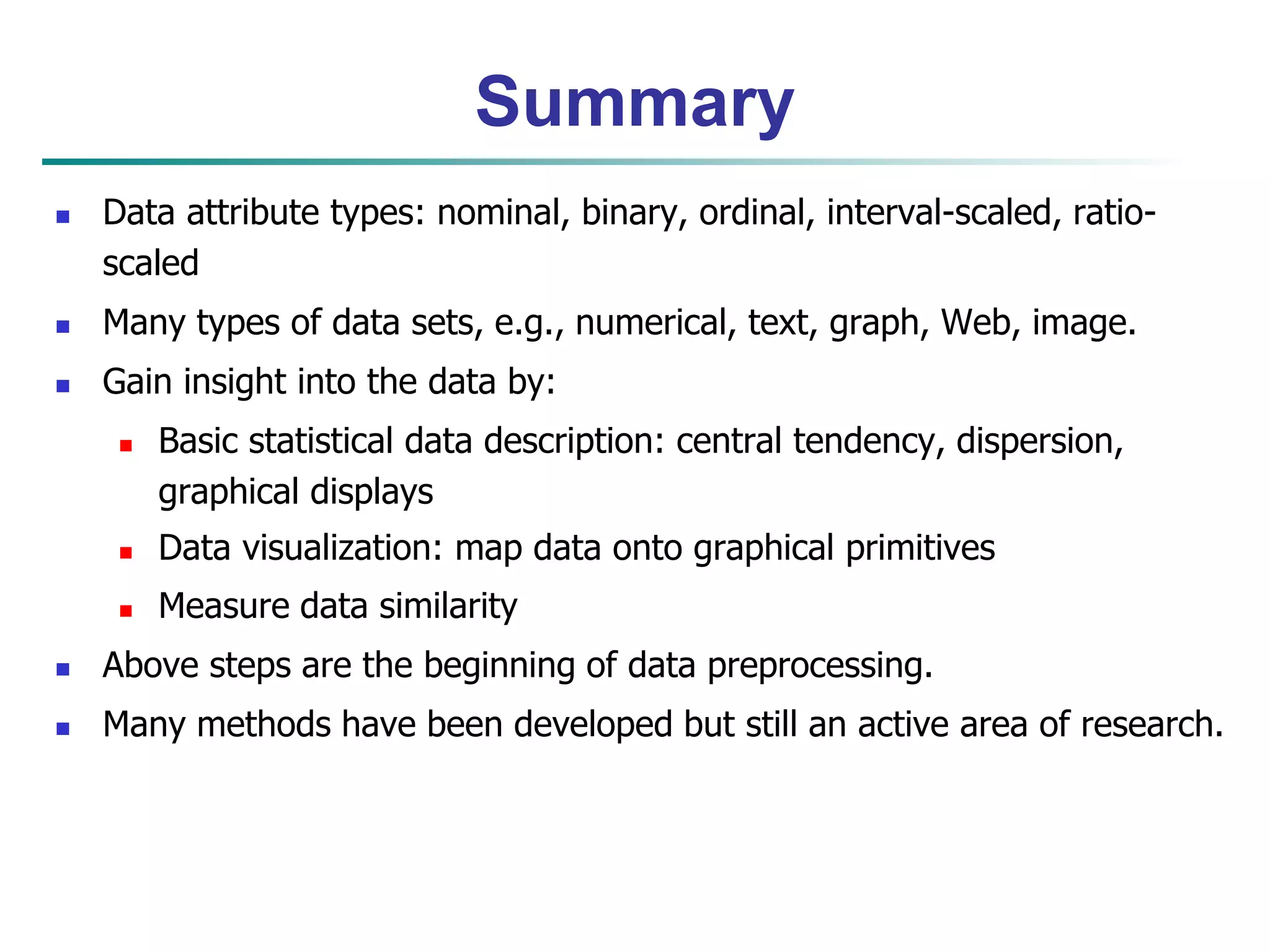
Summary
 Data attribute types: nominal, binary, ordinal, interval-scaled, ratio-scaled
 Many types of data sets, e.g., numerical, text, graph, Web, image.
 Gain insight into the data by:
 Basic statistical data description: central tendency, dispersion,
graphical displays
 Data visualization: map data onto graphical primitives
 Measure data similarity
 Above steps are the beginning of data preprocessing.
 Many methods have been developed but still an active area of research.

02 data

In this document

More Related Content

What's hot

Viewers also liked

Similar to 02 data

Recently uploaded

02 data