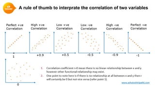
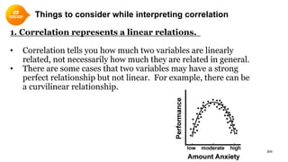
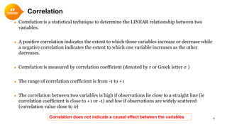
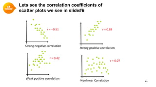
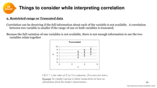
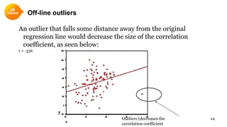
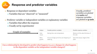
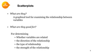
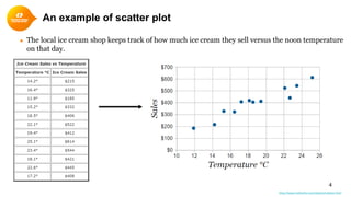
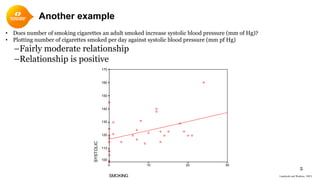
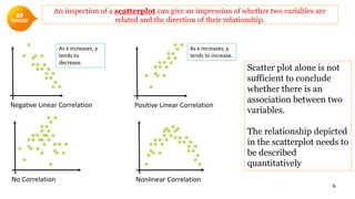
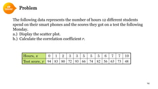
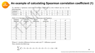
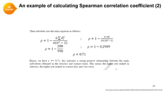
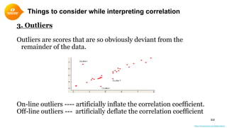
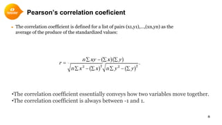
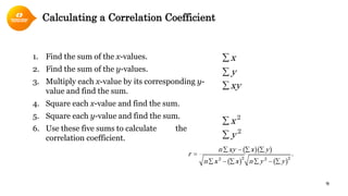
This document discusses correlation and provides examples to illustrate key concepts: 1. Correlation quantifies the linear relationship between two variables and ranges from -1 to 1. Values closer to 1 or -1 indicate a stronger linear relationship. 2. Scatterplots visually depict the relationship and can show if variables are positively or negatively correlated. 3. The Pearson correlation coefficient (r) is a common measure of linear correlation calculated using variables' means, sums, and standard deviations. 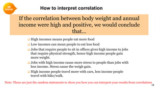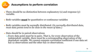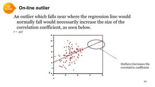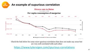4. Correlation only captures linear relationships and does not prove causation between variables. Additional analysis is needed to interpret correlated variables.

1. Lecture:
CORRELATION
Chaudhary Awais Salman
Doctoral Researcher in Future Energy
Course instructor
School of Business, Society and Engineering
Fuuture Energy – Centre of Excellence
Email: Chaudhary.awais.salman@mdh.se

2. Response and predictor variables
● Response or dependant variables
● Variables that are ”observed” or ”measured”
● Predictor variable or independent variables or explanatory variables
● Variables that affect the response
● Usually set by experimenter
Couple of examples
2
https://bit.ly/2MZOIdv
Usually, predictor
variables are plotted
at x-axis and
response variables
are plotted on y-axis
Can a relationship be developed to predict what happens to y as x changes (ie what happens
to the dependent variable as the independent variable changes)?

3. 3
Scatterplots
• What are they?
A graphical tool for examining the relationship between
variables
• What are they good for?
For determining
• Whether variables are related
• the direction of the relationship
• the type of relationship
• the strength of the relationship

4. An example of scatter plot
● The local ice cream shop keeps track of how much ice cream they sell versus the noon temperature
on that day.
4
https://www.mathsisfun.com/data/correlation.html

5. SMOKING
3020100
SYSTOLIC
170
160
150
140
130
120
110
100
Another example
5
• Does number of smoking cigarettes an adult smoked increase systolic blood pressure (mm of Hg)?
• Plotting number of cigarettes smoked per day against systolic blood pressure (mm pf Hg)
–Fairly moderate relationship
–Relationship is positive
Landwehr and Watkins, 1987)

6. An inspection of a scatterplot can give an impression of whether two variables are
related and the direction of their relationship.
6
Scatter plot alone is not
sufficient to conclude
whether there is an
association between two
variables.
The relationship depicted
in the scatterplot needs to
be described
quantitatively
x
y
Negative Linear Correlation
x
y
No Correlation
x
y
Positive Linear Correlation
x
y
Nonlinear Correlation
As x increases, y
tends to
decrease.
As x increases, y
tends to increase.

7. Correlation
● Correlation is a statistical technique to determine the LINEAR relationship between two
variables.
● A positive correlation indicates the extent to which those variables increase or decrease while
a negative correlation indicates the extent to which one variable increases as the other
decreases.
● Correlation is measured by correlation coefficient (denoted by r or Greek letter 𝜎𝜎 )
● The range of correlation coefficient is from -1 to +1
● The correlation between two variables is high if observations lie close to a straight line (ie
correlation coefficient is close to +1 or -1) and low if observations are widely scattered
(correlation value close to 0)
7Correlation does not indicate a causal effect between the variables

8. Pearson’s correlation coeficient
● The correlation coefficient is defined for a list of pairs (x1,y1),…,(xn,yn) as the
average of the produce of the standardized values:
8
•The correlation coefficient essentially conveys how two variables move together.
•The correlation coefficient is always between -1 and 1.
( )( )
( ) ( )2 22 2
.
n xy x y
r
n x x n y y
∑ − ∑ ∑
=
∑ − ∑ ∑ − ∑

9. Calculating a Correlation Coefficient
9
1. Find the sum of the x-values.
2. Find the sum of the y-values.
3. Multiply each x-value by its corresponding y-
value and find the sum.
4. Square each x-value and find the sum.
5. Square each y-value and find the sum.
6. Use these five sums to calculate the
correlation coefficient.
x∑
y∑
xy∑
2
x∑
2
y∑
( )( )
( ) ( )2 22 2
.
n xy x y
r
n x x n y y
∑ − ∑ ∑
=
∑ − ∑ ∑ − ∑

10. Determination of correlation coefficient
10

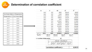
11. Alternative Method
11
Step 1: Find the mean of x, and
the mean of y
Step 2: Subtract the mean of x
from every x value (call them "a"),
do the same for y (call them "b")
Step 3:
Calculate: ab, a2 and b2 for every
value
Step 4: Sum up ab, sum
up a2 and sum up b2
Step 5: Divide the sum of ab by
the square root of [(sum of a2) ×
(sum of b2)]
https://www.mathsisfun.com/data/correlation.html

12. Lets see the correlation coefficients of
scatter plots we see in slide#6
12
x
y
Strong negative correlation
x
y
Weak positive correlation
x
y
Strong positive correlation
x
y
Nonlinear Correlation
r = −0.91 r = 0.88
r = 0.42
r = 0.07

13. A rule of thumb to interprate the correlation of two variables
13

14. Problem
14
Hours, x 0 1 2 3 3 5 5 5 6 7 7 10
Test score, y 94 83 80 72 93 66 74 82 56 63 73 48
The following data represents the number of hours 12 different students
spend on their smart phones and the scores they got on a test the following
Monday.
a.) Display the scatter plot.
b.) Calculate the correlation coefficient r.

15. Spearman correlation coefficient
● Spearman rank correlation developed by Spearman is a non-parametric test
that is used to measure the degree of association between two variables.
● Spearman rank correlation test does not assume any assumptions about the
distribution of the data and is the appropriate correlation analysis when the
variables are measured on a scale that is at least ordinal.
● The following formula is used to calculate the Spearman rank correlation
coefficient:
15
http://www.oicstatcom.org/file/TEXTBOOK-CORRELATION-AND-REGRESSION-ANALYSIS-EGYPT-EN.pdf

16. An example of calculating Spearman correlation coefficient (1)
16
http://www.oicstatcom.org/file/TEXTBOOK-CORRELATION-AND-REGRESSION-ANALYSIS-EGYPT-EN.pdf

17. An example of calculating Spearman correlation coefficient (2)
17
http://www.oicstatcom.org/file/TEXTBOOK-CORRELATION-AND-REGRESSION-ANALYSIS-EGYPT-EN.pdf

18. How to interpret correlation
 High incomes means people eat more food
 Low incomes can mean people to eat less food
 Jobs that require people to sit in offices gives high income to jobs
that require physical strength, hence high income people gain
more weight.
 Jobs with high income cause more stress to people than jobs with
less income. Stress cause the weigh gain.
 High income people travel more with cars, less income people
travel with bike/walk.
18
If the correlation between body weight and annual
income were high and positive, we would conclude
that…
Note: These are just the random statements to show you how you can interpret your results from correlations

19. Assumptions to perform correlation
19
● There should be no distinction between explanatory (x) and response (y)
variable.
● Both variables must be quantitative or continuous variables
● Both variables must be normally distributed. (In normally distributed data,
most data points tend to lie close to the mean of data.)
● Data should be in paired observations
● Every data point must be in pairs. That is, for every observation of the
independent variable, there must be a corresponding observation of the
dependent variable. We cannot compute correlation coefficient if one data set
has 12 observations and the other has 10 observations.
https://helpfulstats.com/assumptions-correlation/

20. Things to consider while interpreting correlation
20
1. Correlation represents a linear relations.
• Correlation tells you how much two variables are linearly
related, not necessarily how much they are related in general.
• There are some cases that two variables may have a strong
perfect relationship but not linear. For example, there can be
a curvilinear relationship.

21. Things to consider while interpreting correlation
21
2. Restricted range or Truncated data
Correlation can be deceiving if the full information about each of the variable is not available. A correlation
between two variable is smaller if the range of one or both variables is truncated.
Because the full variation of one variables is not available, there is not enough information to see the two
variables relate together.
https://www.bauer.uh.edu/rsusmel/phd/ec1-24.pdf

22. Things to consider while interpreting correlation
22
3. Outliers
Outliers are scores that are so obviously deviant from the
remainder of the data.
On-line outliers ---- artificially inflate the correlation coefficient.
Off-line outliers --- artificially deflate the correlation coefficient
https://conversionxl.com/blog/outliers/

23. 23
On-line outlier
An outlier which falls near where the regression line would
normally fall would necessarily increase the size of the
correlation coefficient, as seen below.
r = .457
Outliers (increases the
correlation coefficient

24. 24
Off-line outliers
An outlier that falls some distance away from the original
regression line would decrease the size of the correlation
coefficient, as seen below:
r = .336
Outliers (decreases the
correlation coefficient

25. 25
● 4. Data should be Homoscedastic and not heteroscedastic
Simply put, homoscedasticity means “having the same scatter.” The
points must be about the same distance from the line, as shown in
the picture. The opposite is heteroscedasticity (“different scatter”),
where points are at widely varying distances from the linear line.
https://www.statisticshowto.datasciencecentral.com/homoscedasticity/
Things to consider while interpreting correlation

26. 26
Correlation and Causation
 Two variables with very high correlation coefficient does not
necessarily mean that there is a causation between them .
 A variable can be strongly related to other variable, and still not a
reason for cause. Correlation does not imply causality.
 When there is a correlation between X and Y.
 Does X cause Y or Y cause X, or both?
 Or is there a third variable Z causing both X and Y , and therefore,
X and Y are correlated?

27. An example of supurious correlation
27
https://www.tylervigen.com/spurious-correlations
Check the link below for some more spurious correlation that does not make any sense but
are very well correlated with each other

28. Summary
28
Correlation tell us how strongly two variables are related
Correlation may capture causation between variables but cannot differentiate
from spurious ones.
However, r coefficients are limited in a way as they cannot tell anything about:
What will be the marginal impact of X on Y
Forecasting or modelling with new data points of X
Because of these limitations regression analysis comes, which we will cover in
next lecture