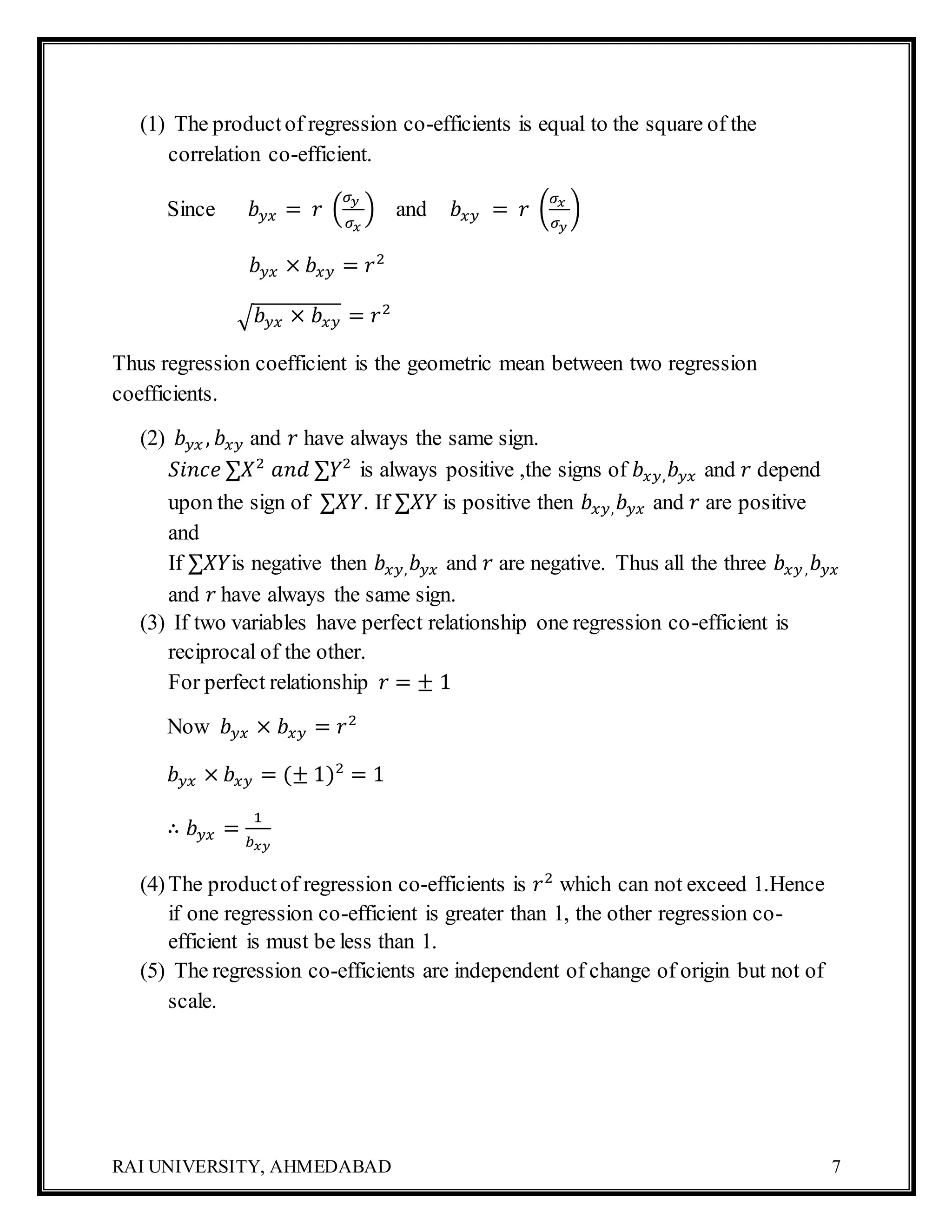
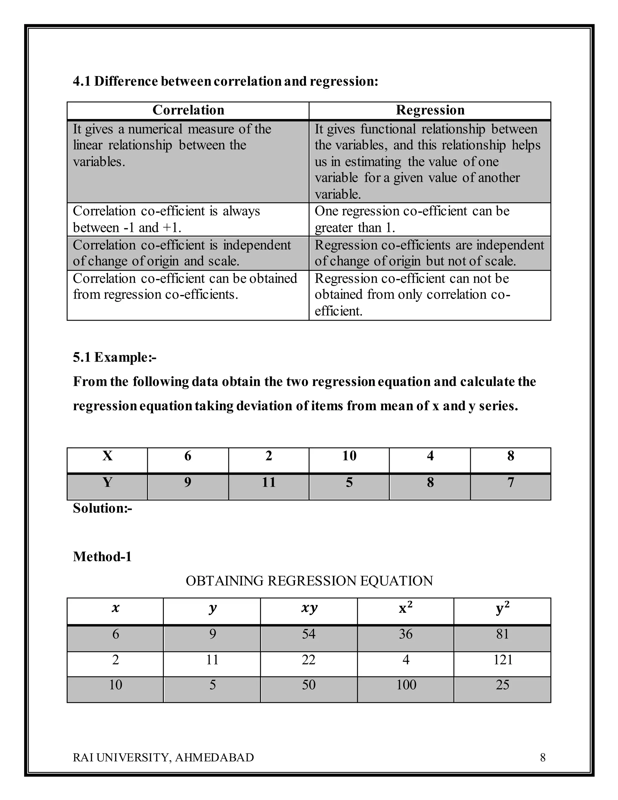
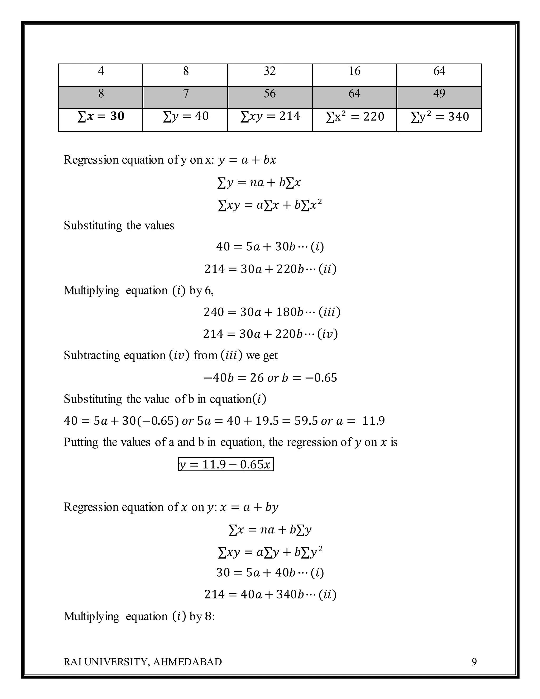
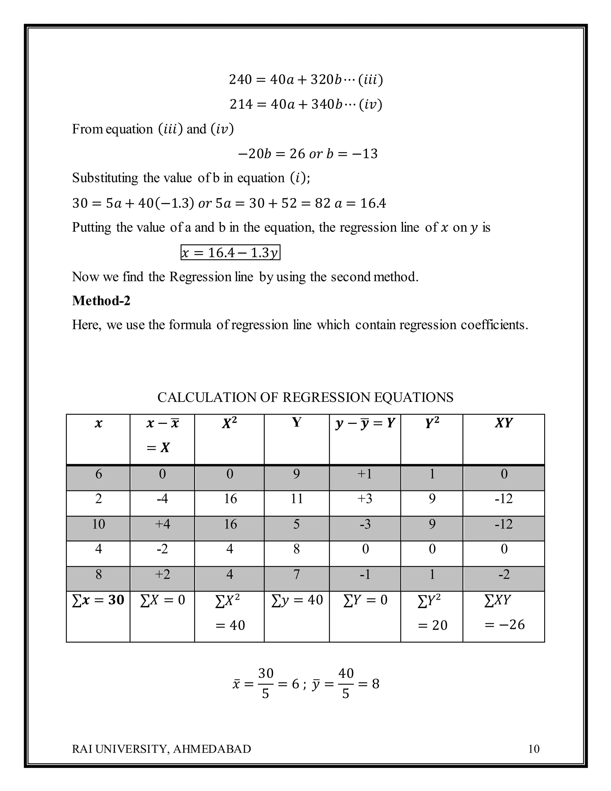
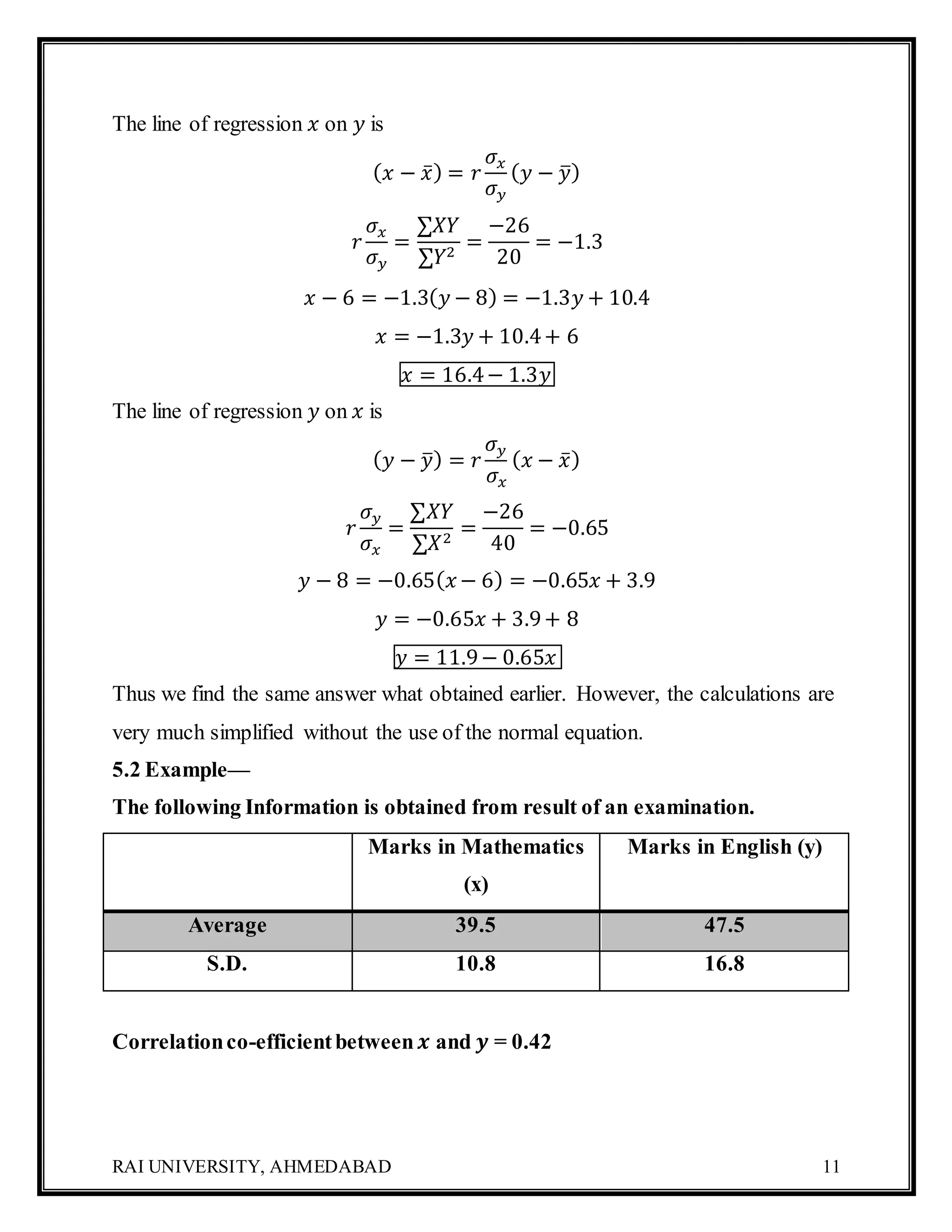
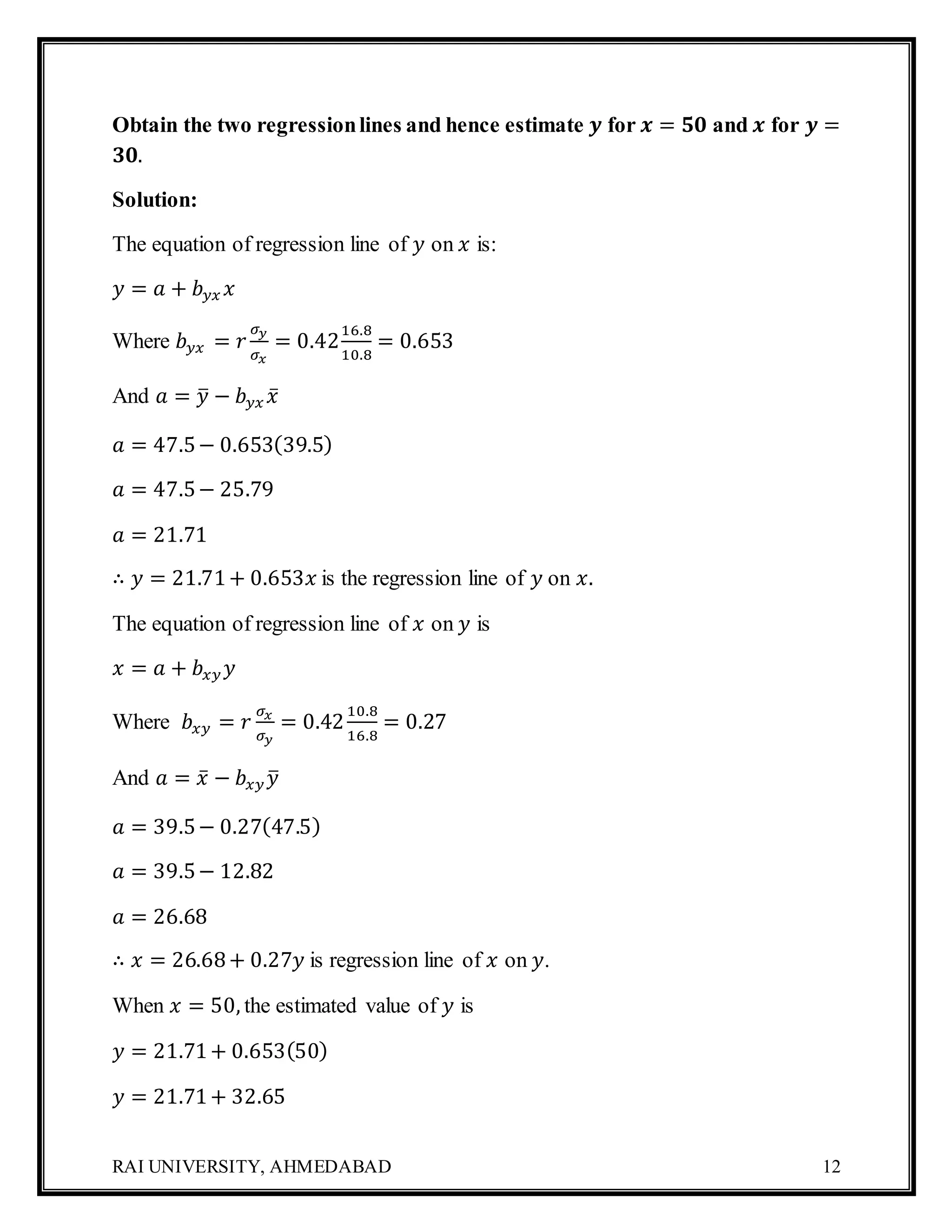
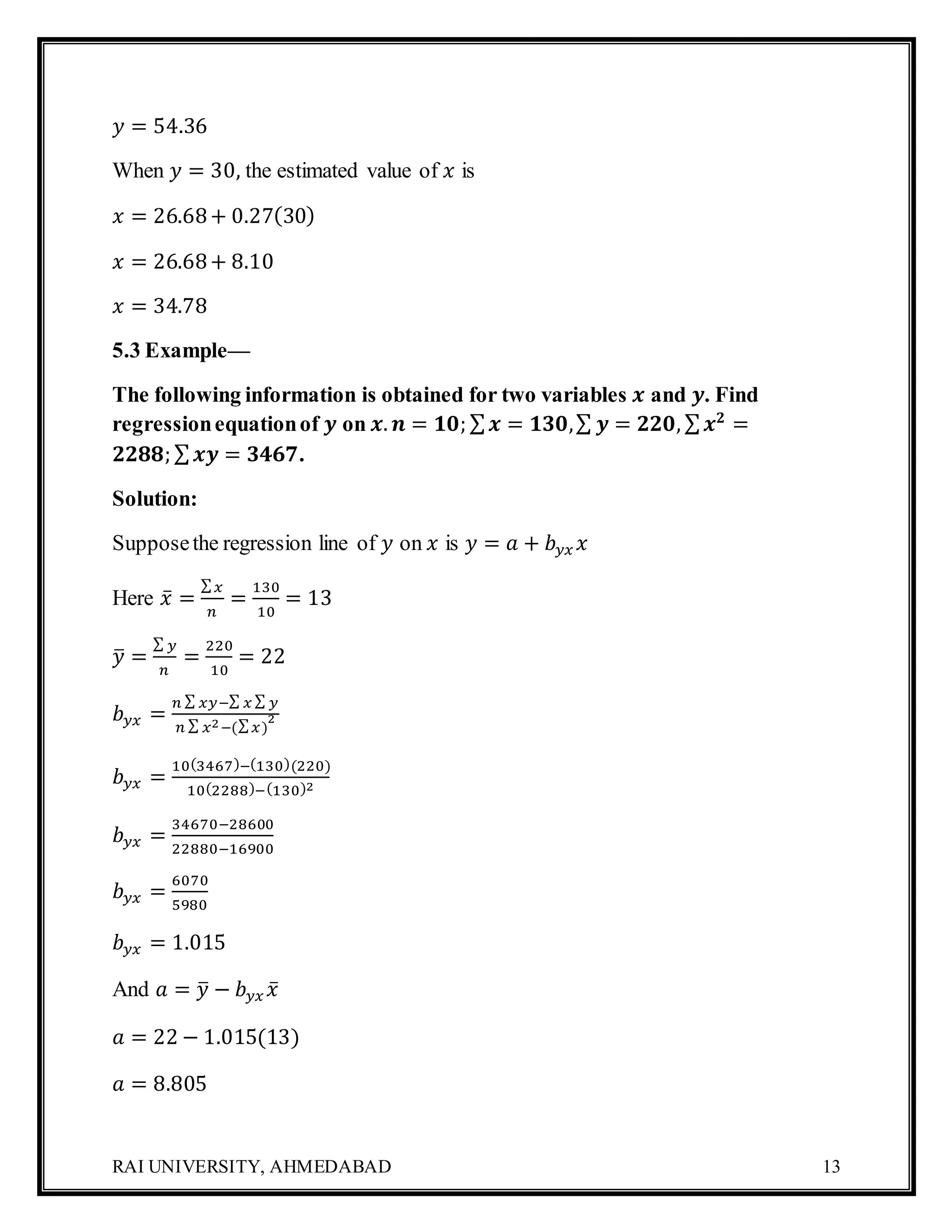
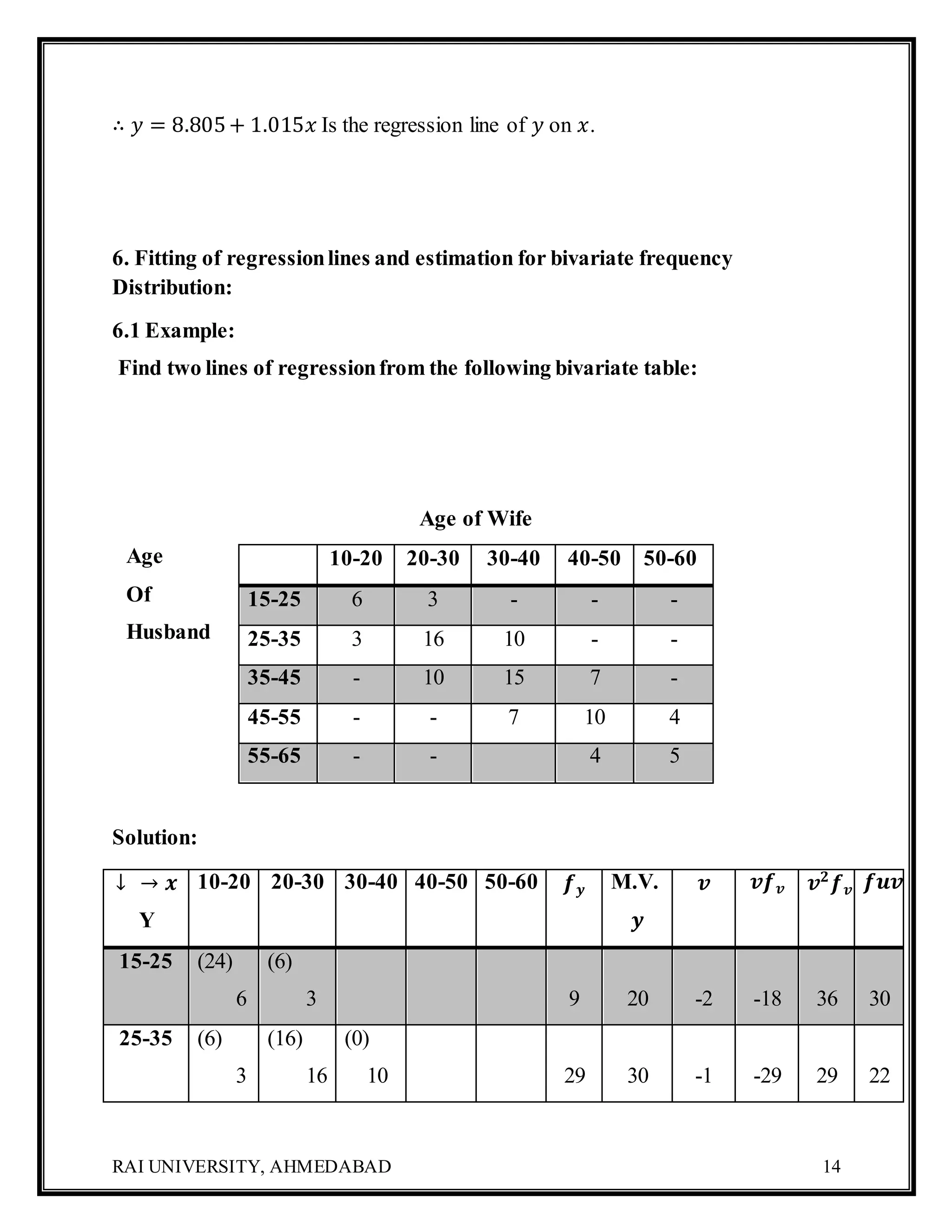
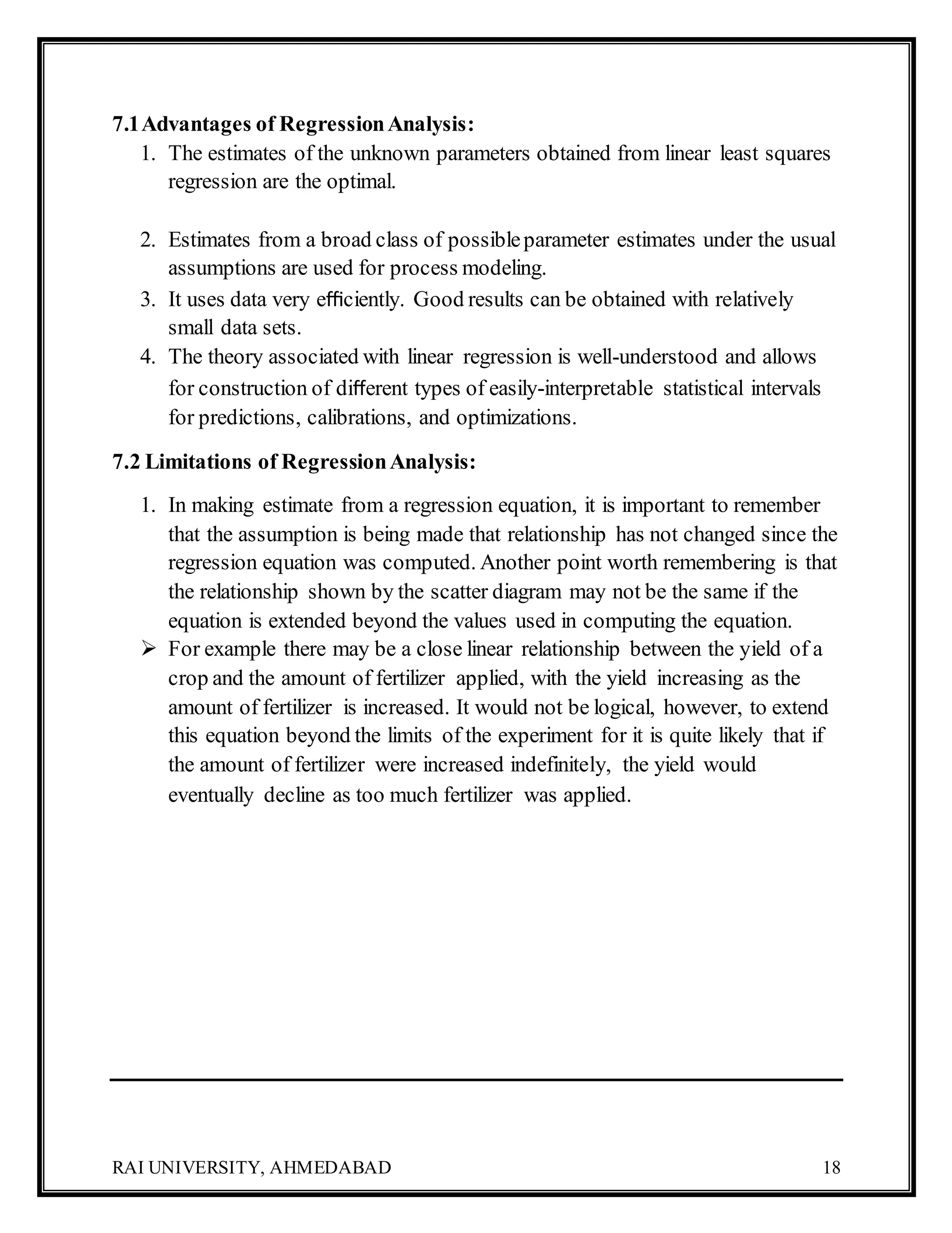
SlideShare a Scribd company logo
RAI UNIVERSITY, AHMEDABAD 1
Course: MCA
Subject: Computer Oriented Numerical
Statistical Methods
Unit-5
RAI UNIVERSITY, AHMEDABAD
RAI UNIVERSITY, AHMEDABAD 2
Unit-V-Regression
Sr.
No.
Name of the Topic Page
No.
1 Introduction and Definition of Regression Analysis 2
2 Regression lines ,Properties and its explanation 3
3 Regression coefficients and its Properties 5
4 Difference between Regression and Correlation 6
5 Example based on the Regression line and Regression Co-
efficients
7
6 Example based on the fitting of regression line and estimation for
bivariate frequency distribution
13
7 Advantage and limitations of Regression Analysis 17
8 References 18
9 Exercise 19
RAI UNIVERSITY, AHMEDABAD 3
Unit-V-Regression
1.1 Introduction:
If two variables are significantly correlated, and if there is some theoretical basis
for doing so, it is possible to predict (estimate) values of one variable from the
other. This observation leads to a very important conceptknown as ‘Regression
Analysis’.
For example, if we know that the advertising and sales are correlated we find out
expected amount of sales for a given advertising expenditure for attaining a given
amount of sales. Similarly if we know the yield of rice and rainfall are closely
related we may find out the amount of rain is required to achieve a certain
production figure.
In general Regression analysis means the estimation or prediction of the unknown
value of one variable from the known value of the other variable. It is one of the
most important statistical tools which is extensively used in almost all sciences –
Natural, Social and Physical.
1.2 Definition:
The dictionary meaning of ‘Regression’ is returning or going back. The term
‘Regression’ is first used by Sir Francis Galton (1822-1911) in 1877 while
studying the relationship between the height of father and sons. This term was
introduced by him in the paper of “Regression towards Mediocrity in healthcare
structure”.
Regression analysis was explained by M. M. Blair as follows:
“Regressionanalysis is a mathematical measure of the average relationship
betweentwo or more variables in terms of the original units of the data”.
RAI UNIVERSITY, AHMEDABAD 4
2.1 RegressionLine:
Regressionline is the line which gives the bestestimate of one variable from the
value of any other given variable.
The regressionline gives the average relationship between the two variables in
mathematical form.
2.2 The Regressionwouldhave the following properties:
a) ∑(𝑦 – 𝑦𝑐) = 0 and b) ∑(𝑦 – 𝑦𝑐)
2
= Minimum
• For two variables X and Y, there are always two lines of regression –
(A)Regressionline of 𝒙 on 𝒚 :
It gives the bestestimate for the value of X for any specific given values of Y
𝒙 = 𝒂 + 𝒃 𝒚
where 𝑎 = 𝑥 - intercept
𝑏 = Slope of the line
𝑥 = Dependent variable
𝑦 = Independent variable
(B) Regressionline of 𝒀 on :
RAI UNIVERSITY, AHMEDABAD 5
• It gives the best estimate for the value of 𝑌 for any specific given values of
𝑋
𝒚 = 𝒂 + 𝒃𝒙
Where 𝑎 = 𝑦 - intercept
𝑏 = Slope of the line
𝑦 = Dependent variable
𝑥= Independent variable
2.3 The Explanation of RegressionLine
• In case of perfect correlation (positive or negative ) the two line of
regression coincide.
• If the two R. line are far from each other then degree of correlation is less,
& vice versa.
• The mean values of 𝑥 & 𝑦 can be obtained as the point of intersection of the
two regression line.
• The higher degree of correlation between the variables, the angle between
the lines is smaller & vice versa.
2.4 RegressionEquation / Line & Method of LeastSquares
2.4.1 RegressionEquationof 𝒚 on 𝒙
𝒚 = 𝒂 + 𝒃𝒙
• In order to obtain the values of ‘𝑎’ & ‘𝑏’
∑𝑦 = 𝑛𝑎 + 𝑏∑𝑥
∑𝑥𝑦 = 𝑎∑𝑥 + 𝑏∑𝑥2
2.4.2 RegressionEquationof 𝒙 on
𝒙 = 𝒄 + 𝒅𝒚
RAI UNIVERSITY, AHMEDABAD 6
• In order to obtain the values of ‘𝑐’ & ‘𝑑’
∑𝑥 = 𝑛𝑐 + 𝑑∑𝑦
∑𝑥𝑦 = 𝑐∑𝑦 + 𝑑∑𝑦2
3.1 RegressionCoefficients:
The regression coefficient between two variables is a numerical measure showing
the change in the value of one variable for a unit change in the value of the other
variable.
3.1.1 Formula for finding regressioncoefficient 𝒃 𝒚𝒙:
Regression Equation of y on x:
𝑦 – 𝑦̅ = 𝑏 𝑦𝑥 (𝑥 – 𝑥̅)
𝑏 𝑦𝑥 =
∑𝑋𝑌
∑𝑋2
𝑏 𝑦𝑥 = 𝑟 (
𝜎 𝑦
𝜎𝑥
)
Also by using the formula of 𝑟, 𝜎𝑥 𝑎𝑛𝑑 𝜎 𝑦 we get 𝑏 𝑦𝑥 =
𝑛 ∑ 𝑥𝑦−∑ 𝑥 ∑ 𝑦
𝑛 ∑ 𝑥2−(∑ 𝑥)
2
3.1.2 Formula for finding regressioncoefficient 𝒃 𝒙𝒚:
Regression Equation of x on y:
𝑥 – 𝑥̅ = 𝑏𝑥𝑦 (𝑦 – 𝑦̅)
𝑏𝑥𝑦 =
∑𝑋𝑌
∑𝑌2
𝑏𝑥𝑦 = 𝑟 (
𝜎𝑥
𝜎 𝑦
)
Also by using the formula of 𝑟, 𝜎𝑥 𝑎𝑛𝑑 𝜎 𝑦 we get 𝑏𝑥𝑦 =
𝑛 ∑ 𝑥𝑦−∑ 𝑥 ∑ 𝑦
𝑛 ∑ 𝑦2−(∑ 𝑦)
2
3.2 Properties of Regressionco-efficients:
RAI UNIVERSITY, AHMEDABAD 7
(1) The productof regression co-efficients is equal to the square of the
correlation co-efficient.
Since 𝑏 𝑦𝑥 = 𝑟 (
𝜎 𝑦
𝜎 𝑥
) and 𝑏𝑥𝑦 = 𝑟 (
𝜎 𝑥
𝜎 𝑦
)
𝑏 𝑦𝑥 × 𝑏𝑥𝑦 = 𝑟2
√ 𝑏 𝑦𝑥 × 𝑏𝑥𝑦 = 𝑟2
Thus regression coefficient is the geometric mean between two regression
coefficients.
(2) 𝑏 𝑦𝑥 , 𝑏𝑥𝑦 and 𝑟 have always the same sign.
𝑆𝑖𝑛𝑐𝑒 ∑𝑋2
𝑎𝑛𝑑 ∑𝑌2
is always positive ,the signs of 𝑏𝑥𝑦, 𝑏 𝑦𝑥 and 𝑟 depend
upon the sign of ∑𝑋𝑌. If ∑𝑋𝑌 is positive then 𝑏𝑥𝑦, 𝑏 𝑦𝑥 and 𝑟 are positive
and
If ∑𝑋𝑌is negative then 𝑏𝑥𝑦, 𝑏 𝑦𝑥 and 𝑟 are negative. Thus all the three 𝑏𝑥𝑦, 𝑏 𝑦𝑥
and 𝑟 have always the same sign.
(3) If two variables have perfect relationship one regression co-efficient is
reciprocal of the other.
For perfect relationship 𝑟 = ± 1
Now 𝑏 𝑦𝑥 × 𝑏𝑥𝑦 = 𝑟2
𝑏 𝑦𝑥 × 𝑏𝑥𝑦 = (± 1)2
= 1
∴ 𝑏 𝑦𝑥 =
1
𝑏 𝑥𝑦
(4)The productof regression co-efficients is 𝑟2
which can not exceed 1.Hence
if one regression co-efficient is greater than 1, the other regression co-
efficient is must be less than 1.
(5) The regression co-efficients are independent of change of origin but not of
scale.
RAI UNIVERSITY, AHMEDABAD 8
4.1 Difference betweencorrelationand regression:
Correlation Regression
It gives a numerical measure of the
linear relationship between the
variables.
It gives functional relationship between
the variables, and this relationship helps
us in estimating the value of one
variable for a given value of another
variable.
Correlation co-efficient is always
between -1 and +1.
One regression co-efficient can be
greater than 1.
Correlation co-efficient is independent
of change of origin and scale.
Regression co-efficients are independent
of change of origin but not of scale.
Correlation co-efficient can be obtained
from regression co-efficients.
Regression co-efficient can not be
obtained from only correlation co-
efficient.
5.1 Example:-
From the following data obtain the two regressionequation and calculate the
regressionequationtaking deviation of items from mean of x and y series.
X 6 2 10 4 8
Y 9 11 5 8 7
Solution:-
Method-1
OBTAINING REGRESSION EQUATION
𝒙 𝒚 𝒙𝒚 𝐱 𝟐
𝐲 𝟐
6 9 54 36 81
2 11 22 4 121
10 5 50 100 25
RAI UNIVERSITY, AHMEDABAD 9
4 8 32 16 64
8 7 56 64 49
∑𝒙 = 𝟑𝟎 ∑𝑦 = 40 ∑𝑥𝑦 = 214 ∑x2
= 220 ∑y2
= 340
Regression equation of y on x: 𝑦 = 𝑎 + 𝑏𝑥
∑𝑦 = 𝑛𝑎 + 𝑏∑𝑥
∑𝑥𝑦 = 𝑎∑𝑥 + 𝑏∑𝑥2
Substituting the values
40 = 5𝑎 + 30𝑏⋯(𝑖)
214 = 30𝑎 + 220𝑏⋯( 𝑖𝑖)
Multiplying equation (𝑖) by 6,
240 = 30𝑎 + 180𝑏⋯ ( 𝑖𝑖𝑖)
214 = 30𝑎 + 220𝑏⋯( 𝑖𝑣)
Subtracting equation ( 𝑖𝑣) from ( 𝑖𝑖𝑖) we get
−40𝑏 = 26 𝑜𝑟 𝑏 = −0.65
Substituting the value of b in equation( 𝑖)
40 = 5𝑎 + 30(−0.65) 𝑜𝑟 5𝑎 = 40 + 19.5 = 59.5 𝑜𝑟 𝑎 = 11.9
Putting the values of a and b in equation, the regression of 𝑦 on 𝑥 is
𝑦 = 11.9− 0.65𝑥
Regression equation of 𝑥 on 𝑦: 𝑥 = 𝑎 + 𝑏𝑦
∑𝑥 = 𝑛𝑎 + 𝑏∑𝑦
∑𝑥𝑦 = 𝑎∑𝑦 + 𝑏∑𝑦2
30 = 5𝑎 + 40𝑏⋯(𝑖)
214 = 40𝑎 + 340𝑏⋯(𝑖𝑖)
Multiplying equation ( 𝑖) by 8:
RAI UNIVERSITY, AHMEDABAD 10
240 = 40𝑎 + 320𝑏⋯(𝑖𝑖𝑖)
214 = 40𝑎 + 340𝑏⋯(𝑖𝑣)
From equation ( 𝑖𝑖𝑖) and ( 𝑖𝑣)
−20𝑏 = 26 𝑜𝑟 𝑏 = −13
Substituting the value of b in equation ( 𝑖);
30 = 5𝑎 + 40(−1.3) 𝑜𝑟 5𝑎 = 30 + 52 = 82 𝑎 = 16.4
Putting the value of a and b in the equation, the regression line of 𝑥 on 𝑦 is
𝑥 = 16.4− 1.3𝑦
Now we find the Regression line by using the second method.
Method-2
Here, we use the formula of regression line which contain regression coefficients.
CALCULATION OF REGRESSION EQUATIONS
𝒙 𝒙 − 𝒙̅
= 𝑿
𝑿 𝟐 Y 𝒚 − 𝒚̅ = 𝒀 𝒀 𝟐 𝑿𝒀
6 0 0 9 +1 1 0
2 -4 16 11 +3 9 -12
10 +4 16 5 -3 9 -12
4 -2 4 8 0 0 0
8 +2 4 7 -1 1 -2
∑𝒙 = 𝟑𝟎 ∑𝑋 = 0 ∑𝑋2
= 40
∑𝑦 = 40 ∑𝑌 = 0 ∑𝑌2
= 20
∑𝑋𝑌
= −26
𝑥̅ =
30
5
= 6 ; 𝑦̅ =
40
5
= 8
RAI UNIVERSITY, AHMEDABAD 11
The line of regression 𝑥 on 𝑦 is
( 𝑥 − 𝑥̅) = 𝑟
𝜎𝑥
𝜎 𝑦
( 𝑦 − 𝑦̅)
𝑟
𝜎𝑥
𝜎 𝑦
=
∑𝑋𝑌
∑𝑌2
=
−26
20
= −1.3
𝑥 − 6 = −1.3( 𝑦 − 8) = −1.3𝑦 + 10.4
𝑥 = −1.3𝑦 + 10.4+ 6
𝑥 = 16.4− 1.3𝑦
The line of regression 𝑦 on 𝑥 is
( 𝑦 − 𝑦̅) = 𝑟
𝜎 𝑦
𝜎𝑥
( 𝑥 − 𝑥̅)
𝑟
𝜎 𝑦
𝜎𝑥
=
∑𝑋𝑌
∑𝑋2
=
−26
40
= −0.65
𝑦 − 8 = −0.65( 𝑥 − 6) = −0.65𝑥 + 3.9
𝑦 = −0.65𝑥 + 3.9+ 8
𝑦 = 11.9− 0.65𝑥
Thus we find the same answer what obtained earlier. However, the calculations are
very much simplified without the use of the normal equation.
5.2 Example—
The following Information is obtained from result of an examination.
Marks in Mathematics
(x)
Marks in English (y)
Average 39.5 47.5
S.D. 10.8 16.8
Correlationco-efficientbetween 𝒙 and 𝒚 = 0.42
RAI UNIVERSITY, AHMEDABAD 12
Obtain the two regressionlines and hence estimate 𝒚 for 𝒙 = 𝟓𝟎 and 𝒙 for 𝒚 =
𝟑𝟎.
Solution:
The equation of regression line of 𝑦 on 𝑥 is:
𝑦 = 𝑎 + 𝑏 𝑦𝑥 𝑥
Where 𝑏 𝑦𝑥 = 𝑟
𝜎 𝑦
𝜎 𝑥
= 0.42
16.8
10.8
= 0.653
And 𝑎 = 𝑦̅ − 𝑏 𝑦𝑥 𝑥̅
𝑎 = 47.5− 0.653(39.5)
𝑎 = 47.5− 25.79
𝑎 = 21.71
∴ 𝑦 = 21.71+ 0.653𝑥 is the regression line of 𝑦 on 𝑥.
The equation of regression line of 𝑥 on 𝑦 is
𝑥 = 𝑎 + 𝑏𝑥𝑦 𝑦
Where 𝑏𝑥𝑦 = 𝑟
𝜎 𝑥
𝜎 𝑦
= 0.42
10.8
16.8
= 0.27
And 𝑎 = 𝑥̅ − 𝑏𝑥𝑦 𝑦̅
𝑎 = 39.5− 0.27(47.5)
𝑎 = 39.5− 12.82
𝑎 = 26.68
∴ 𝑥 = 26.68+ 0.27𝑦 is regression line of 𝑥 on 𝑦.
When 𝑥 = 50, the estimated value of 𝑦 is
𝑦 = 21.71+ 0.653(50)
𝑦 = 21.71+ 32.65
RAI UNIVERSITY, AHMEDABAD 13
𝑦 = 54.36
When 𝑦 = 30, the estimated value of 𝑥 is
𝑥 = 26.68+ 0.27(30)
𝑥 = 26.68+ 8.10
𝑥 = 34.78
5.3 Example—
The following information is obtained for two variables 𝒙 and 𝒚. Find
regressionequationof 𝒚 on 𝒙. 𝒏 = 𝟏𝟎; ∑ 𝒙 = 𝟏𝟑𝟎,∑ 𝒚 = 𝟐𝟐𝟎, ∑ 𝒙 𝟐
=
𝟐𝟐𝟖𝟖; ∑ 𝒙𝒚 = 𝟑𝟒𝟔𝟕.
Solution:
Supposethe regression line of 𝑦 on 𝑥 is 𝑦 = 𝑎 + 𝑏 𝑦𝑥 𝑥
Here 𝑥̅ =
∑ 𝑥
𝑛
=
130
10
= 13
𝑦̅ =
∑ 𝑦
𝑛
=
220
10
= 22
𝑏 𝑦𝑥 =
𝑛 ∑ 𝑥𝑦−∑ 𝑥 ∑ 𝑦
𝑛 ∑ 𝑥2−(∑ 𝑥)
2
𝑏 𝑦𝑥 =
10(3467)−(130)(220)
10(2288)−(130)2
𝑏 𝑦𝑥 =
34670−28600
22880−16900
𝑏 𝑦𝑥 =
6070
5980
𝑏 𝑦𝑥 = 1.015
And 𝑎 = 𝑦̅ − 𝑏 𝑦𝑥 𝑥̅
𝑎 = 22 − 1.015(13)
𝑎 = 8.805
RAI UNIVERSITY, AHMEDABAD 14
∴ 𝑦 = 8.805+ 1.015𝑥 Is the regression line of 𝑦 on 𝑥.
6. Fitting of regressionlines and estimation for bivariate frequency
Distribution:
6.1 Example:
Find two lines of regressionfrom the following bivariate table:
Age of Wife
Age
Of
Husband
Solution:
↓ → 𝒙
Y
10-20 20-30 30-40 40-50 50-60 𝒇 𝒚 M.V.
𝒚
𝒗 𝒗𝒇 𝒗 𝒗 𝟐
𝒇 𝒗 𝒇𝒖𝒗
15-25 (24)
6
(6)
3 9 20 -2 -18 36 30
25-35 (6)
3
(16)
16
(0)
10 29 30 -1 -29 29 22
10-20 20-30 30-40 40-50 50-60
15-25 6 3 - - -
25-35 3 16 10 - -
35-45 - 10 15 7 -
45-55 - - 7 10 4
55-65 - - 4 5
RAI UNIVERSITY, AHMEDABAD 15
35-45 (0)
10
(0)
15
(0)
7 32 40 0 0 0 0
45-55 (0)
7
(10)
10
(8)
4 21 50 1 21 21 18
55-65 (8)
4
(20)
5 9 60 2 18 36 28
𝒇 𝒙 9 29 32 21 9 100 -8 122 98
M.V. 𝒙 15 25 35 45 55
𝒖 -2 -1 0 1 2
𝒖𝒇 𝒖 -18 -29 0 21 18 -8
𝒖 𝟐
𝒇 𝒖 36 29 0 21 36 122
𝒇𝒖𝒗 30 22 0 18 28 98
Here 𝑋̅ = 𝐴 +
∑ 𝑢𝑓𝑢
𝑛
× 𝐶𝑥
𝑋̅ = 35 +
−8
100
× 10
𝑋̅ = 34.2
𝑌̅ = 𝐵 +
∑ 𝑣𝑓𝑣
𝑛
× 𝐶𝑦
𝑌̅ = 40 +
−8
100
× 10
𝑌̅ = 39.2
Supposethe regression equation of 𝑦 on 𝑥 is
𝑦 = 𝑎 + 𝑏 𝑦𝑥 𝑥
Where, 𝑏 𝑦𝑥 =
𝑛 ∑ 𝑓𝑢𝑣−∑ 𝑢𝑓𝑢 ∑ 𝑣𝑓𝑣
𝑛 ∑ 𝑢2 𝑓𝑢−(∑ 𝑢𝑓𝑢)
2 ×
𝐶 𝑦
𝐶 𝑥
RAI UNIVERSITY, AHMEDABAD 16
𝑏 𝑦𝑥 =
100×98−(−8)(−8)
100×122−(−8)2
×
10
10
𝑏 𝑦𝑥 =
9800−64
12200−64
× 1
𝑏 𝑦𝑥 =
9736
12136
𝑏 𝑦𝑥 = 0.802
And, 𝑎 = 𝑦̅ − 𝑏 𝑦𝑥 𝑥̅
𝑎 = 39.2− 0.802(34.2)
𝑎 = 39.2− 27.43
𝑎 = 11.77
∴ 𝑦 = 11.77+ 0.802𝑥 is the regression line of 𝑦 on 𝑥.
Now supposethe regression line of 𝑥 on 𝑦 is
𝑥 = 𝑎 + 𝑏𝑥𝑦 𝑦
Where 𝑏𝑥𝑦 =
𝑛 ∑ 𝑓𝑢𝑣−∑ 𝑢𝑓𝑢 ∑ 𝑣𝑓𝑣
𝑛 ∑ 𝑣2 𝑓𝑣−(∑ 𝑣𝑓𝑣)
2 ×
𝐶 𝑥
𝐶 𝑦
𝑏𝑥𝑦 =
9736
100×122−(−8)2
×
10
10
𝑏𝑥𝑦 = 0.802
And 𝑎 = 𝑥̅ − 𝑏𝑥𝑦 𝑦̅
𝑎 = 34.2− 0.802(39.2)
𝑎 = 34.2− 31.44
𝑎 = 2.76
∴ 𝑥 = 2.76 + 0.802𝑦 is the regression line of 𝑥 on 𝑦.
6.2 Example—
RAI UNIVERSITY, AHMEDABAD 17
Calculate 𝒃 𝒚𝒙, 𝒃 𝒙𝒚& 𝑟 using the following:
Given Value Estimated Value
𝒙 = 𝟏𝟎 𝑦 = 22
𝒙 = 𝟐𝟎 𝑦 = 34
𝒚 = 𝟑𝟎 𝑥 = 17
𝒚 = 𝟓𝟎 𝑥 = 23
Solution:
Let the regression equation of 𝑦 on 𝑥 be 𝑦 = 𝑎 + 𝑏 𝑦𝑥 𝑦
∴ 22 = 𝑎 + 𝑏 𝑦𝑥 . 10
34 = 𝑎 + 𝑏 𝑦𝑥 . 20
_____________________
−12 = −10𝑏 𝑦𝑥
∴ 𝑏 𝑦𝑥 = 1.2
Let the regression equation of 𝑥 on 𝑦 be 𝑥 = 𝑎 + 𝑏𝑥𝑦 𝑦
∴ 17 = 𝑎 + 𝑏𝑥𝑦. 30
23 = 𝑎 + 𝑏𝑥𝑦. 50
_______________________
−6 = −𝑏𝑥𝑦. 20
𝑏𝑥𝑦 =
6
20
= 0.3
Now 𝑟 = √ 𝑏 𝑦𝑥. 𝑏𝑥𝑦
𝑟 = √(1.2)(0.3)
𝑟 = √0.36
𝑟 = 0.6
RAI UNIVERSITY, AHMEDABAD 18
7.1Advantages of RegressionAnalysis:
1. The estimates of the unknown parameters obtained from linear least squares
regression are the optimal.
2. Estimates from a broad class of possibleparameter estimates under the usual
assumptions are used for process modeling.
3. It uses data very efficiently. Good results can be obtained with relatively
small data sets.
4. The theory associated with linear regression is well-understood and allows
for construction of different types of easily-interpretable statistical intervals
for predictions, calibrations, and optimizations.
7.2 Limitations of RegressionAnalysis:
1. In making estimate from a regression equation, it is important to remember
that the assumption is being made that relationship has not changed since the
regression equation was computed. Another point worth remembering is that
the relationship shown by the scatter diagram may not be the same if the
equation is extended beyond the values used in computing the equation.
 For example there may be a close linear relationship between the yield of a
crop and the amount of fertilizer applied, with the yield increasing as the
amount of fertilizer is increased. It would not be logical, however, to extend
this equation beyond the limits of the experiment for it is quite likely that if
the amount of fertilizer were increased indefinitely, the yield would
eventually decline as too much fertilizer was applied.
RAI UNIVERSITY, AHMEDABAD 19
Reference BookandWebsite Name:
1. Statistical Methods by S.P.Gupat
2. Business statistics by R.S.Bardwaj
3. Business statistics ( B.S. Shah Prakashan)
4. www.answers.com/Q/What_is_the_advantages_and_disadvantages_of_mult
iple_regression_analysis
5. http://www.biomedware.com/files/documentation/spacestat/Statistics/Multiv
ariate_Modeling/Regression/regression_line.png
RAI UNIVERSITY, AHMEDABAD 20
EXERCISE
Q-1. Evaluate the following Questions:
1. Find the equations of regression lines from the following data and also
estimate 𝑦 for 𝑥 = 1 and 𝑥 for 𝑦 = 4.
𝒙: 3 2 -1 6 4 -2 5 7
𝒚: 5 13 12 -1 2 20 0 -3
2. Find regression co-efficients from the following data:
𝒙: 21 22 23 24 25 26 27 28 29 30
𝒚: 17 19 19 20 23 24 27 26 28 27
3. Obtain two regression lines from the following bivariate table:
Height Weight
90-100 100-110 110-120 120-130
50-55 4 7 5 2
55-60 6 10 7 4
60-65 6 12 10 7
65-70 3 8 6 3
4. The two regression lines are 𝑥 + 2𝑦 − 5 = 0 and 2𝑥 + 3𝑦 − 8 = 0and
𝜎𝑥
2
=12, find 𝑥̅ ,𝑦̅,𝜎 𝑦
2
𝑎𝑛𝑑 𝑟.
RAI UNIVERSITY, AHMEDABAD 21

More Related Content

What's hot

Crout s method for solving system of linear equations
Crout s method for solving system of linear equationsCrout s method for solving system of linear equations
Crout s method for solving system of linear equations
Sugathan Velloth
 
Specific topics in optimisation
Specific topics in optimisationSpecific topics in optimisation
Specific topics in optimisation
Farzad Javidanrad
 
Systems of equations alg1
Systems of equations alg1Systems of equations alg1
Systems of equations alg1Hazel Joy Chong
 
Matrix
MatrixMatrix
Linear and non linear equation
Linear and non linear equationLinear and non linear equation
Linear and non linear equation
Harshana Madusanka Jayamaha
 
Lecture 4
Lecture 4Lecture 4
Statistics (recap)
Statistics (recap)Statistics (recap)
Statistics (recap)
Farzad Javidanrad
 
System of linear equations
System of linear equationsSystem of linear equations
System of linear equations
Diler4
 
Math 8 - Linear Functions
Math 8 - Linear FunctionsMath 8 - Linear Functions
Math 8 - Linear Functions
Carlo Luna
 
Systems of 3 Equations in 3 Variables
Systems of 3 Equations in 3 VariablesSystems of 3 Equations in 3 Variables
Systems of 3 Equations in 3 Variables
Mid Michigan Community College
 
Comparative analysis of x^3+y^3=z^3 and x^2+y^2=z^2 in the Interconnected Sets
Comparative analysis of x^3+y^3=z^3 and x^2+y^2=z^2 in the Interconnected Sets Comparative analysis of x^3+y^3=z^3 and x^2+y^2=z^2 in the Interconnected Sets
Comparative analysis of x^3+y^3=z^3 and x^2+y^2=z^2 in the Interconnected Sets
Vladimir Godovalov
 
Systemsof3 equations
Systemsof3 equationsSystemsof3 equations
Systemsof3 equations
gandhinagar
 
Sytems of linear equation
Sytems of linear equationSytems of linear equation
Sytems of linear equation
Franz Uy
 
System Of Linear Equations
System Of Linear EquationsSystem Of Linear Equations
System Of Linear Equations
saahil kshatriya
 
Math 8 - Linear Inequalities in Two Variables
Math 8 - Linear Inequalities in Two VariablesMath 8 - Linear Inequalities in Two Variables
Math 8 - Linear Inequalities in Two Variables
Carlo Luna
 
System of equations
System of equationsSystem of equations
System of equationsmariacadena
 
1.1 Linear Equations
1.1 Linear Equations1.1 Linear Equations
1.1 Linear Equations
smiller5
 

What's hot (20)

Crout s method for solving system of linear equations
Crout s method for solving system of linear equationsCrout s method for solving system of linear equations
Crout s method for solving system of linear equations
 
Specific topics in optimisation
Specific topics in optimisationSpecific topics in optimisation
Specific topics in optimisation
 
Systems of equations alg1
Systems of equations alg1Systems of equations alg1
Systems of equations alg1
 
Matrix
MatrixMatrix
Matrix
 
Linear and non linear equation
Linear and non linear equationLinear and non linear equation
Linear and non linear equation
 
Lecture 4
Lecture 4Lecture 4
Lecture 4
 
Statistics (recap)
Statistics (recap)Statistics (recap)
Statistics (recap)
 
System of linear equations
System of linear equationsSystem of linear equations
System of linear equations
 
Math 8 - Linear Functions
Math 8 - Linear FunctionsMath 8 - Linear Functions
Math 8 - Linear Functions
 
Systems of 3 Equations in 3 Variables
Systems of 3 Equations in 3 VariablesSystems of 3 Equations in 3 Variables
Systems of 3 Equations in 3 Variables
 
Comparative analysis of x^3+y^3=z^3 and x^2+y^2=z^2 in the Interconnected Sets
Comparative analysis of x^3+y^3=z^3 and x^2+y^2=z^2 in the Interconnected Sets Comparative analysis of x^3+y^3=z^3 and x^2+y^2=z^2 in the Interconnected Sets
Comparative analysis of x^3+y^3=z^3 and x^2+y^2=z^2 in the Interconnected Sets
 
Systemsof3 equations
Systemsof3 equationsSystemsof3 equations
Systemsof3 equations
 
Linear algebra03fallleturenotes01
Linear algebra03fallleturenotes01Linear algebra03fallleturenotes01
Linear algebra03fallleturenotes01
 
Sytems of linear equation
Sytems of linear equationSytems of linear equation
Sytems of linear equation
 
Systems of equations and matricies
Systems of equations and matriciesSystems of equations and matricies
Systems of equations and matricies
 
System Of Linear Equations
System Of Linear EquationsSystem Of Linear Equations
System Of Linear Equations
 
Math 8 - Linear Inequalities in Two Variables
Math 8 - Linear Inequalities in Two VariablesMath 8 - Linear Inequalities in Two Variables
Math 8 - Linear Inequalities in Two Variables
 
System of equations
System of equationsSystem of equations
System of equations
 
1.1 Linear Equations
1.1 Linear Equations1.1 Linear Equations
1.1 Linear Equations
 
Gauss sediel
Gauss sedielGauss sediel
Gauss sediel
 

Viewers also liked

MCA_UNIT-3_Computer Oriented Numerical Statistical Methods
MCA_UNIT-3_Computer Oriented Numerical Statistical MethodsMCA_UNIT-3_Computer Oriented Numerical Statistical Methods
MCA_UNIT-3_Computer Oriented Numerical Statistical Methods
Rai University
 
Mm unit 4point2
Mm unit 4point2Mm unit 4point2
Mm unit 4point2
Rai University
 
Mca 2 sem u-1 iintroduction
Mca 2 sem u-1 iintroductionMca 2 sem u-1 iintroduction
Mca 2 sem u-1 iintroduction
Rai University
 
MITCOE 2011-12 conm-submission
MITCOE 2011-12 conm-submissionMITCOE 2011-12 conm-submission
MITCOE 2011-12 conm-submissionAshutosh Katti
 
A time study in numerical methods programming
A time study in numerical methods programmingA time study in numerical methods programming
A time study in numerical methods programming
Glen Alleman
 
Bisection & Regual falsi methods
Bisection & Regual falsi methodsBisection & Regual falsi methods
Bisection & Regual falsi methods
Divya Bhatia
 
BCA_Semester-II-Discrete Mathematics_unit-iv Graph theory
BCA_Semester-II-Discrete Mathematics_unit-iv Graph theoryBCA_Semester-II-Discrete Mathematics_unit-iv Graph theory
BCA_Semester-II-Discrete Mathematics_unit-iv Graph theory
Rai University
 
BSC_COMPUTER _SCIENCE_UNIT-5_DISCRETE MATHEMATICS
BSC_COMPUTER _SCIENCE_UNIT-5_DISCRETE MATHEMATICSBSC_COMPUTER _SCIENCE_UNIT-5_DISCRETE MATHEMATICS
BSC_COMPUTER _SCIENCE_UNIT-5_DISCRETE MATHEMATICS
Rai University
 
BSC_Computer Science_Discrete Mathematics_Unit-I
BSC_Computer Science_Discrete Mathematics_Unit-IBSC_Computer Science_Discrete Mathematics_Unit-I
BSC_Computer Science_Discrete Mathematics_Unit-I
Rai University
 
Btech_II_ engineering mathematics_unit5
Btech_II_ engineering mathematics_unit5Btech_II_ engineering mathematics_unit5
Btech_II_ engineering mathematics_unit5
Rai University
 
B.tech ii unit-4 material vector differentiation
B.tech ii unit-4 material vector differentiationB.tech ii unit-4 material vector differentiation
B.tech ii unit-4 material vector differentiation
Rai University
 
Unit 1 Introduction
Unit 1 IntroductionUnit 1 Introduction
Unit 1 Introduction
Rai University
 
B.tech ii unit-5 material vector integration
B.tech ii unit-5 material vector integrationB.tech ii unit-5 material vector integration
B.tech ii unit-5 material vector integration
Rai University
 
Btech_II_ engineering mathematics_unit4
Btech_II_ engineering mathematics_unit4Btech_II_ engineering mathematics_unit4
Btech_II_ engineering mathematics_unit4
Rai University
 
B.Tech-II_Unit-III
B.Tech-II_Unit-IIIB.Tech-II_Unit-III
B.Tech-II_Unit-IIIKundan Kumar
 
BSC_COMPUTER _SCIENCE_UNIT-4_DISCRETE MATHEMATICS
BSC_COMPUTER _SCIENCE_UNIT-4_DISCRETE MATHEMATICSBSC_COMPUTER _SCIENCE_UNIT-4_DISCRETE MATHEMATICS
BSC_COMPUTER _SCIENCE_UNIT-4_DISCRETE MATHEMATICS
Rai University
 

Viewers also liked (20)

MCA_UNIT-3_Computer Oriented Numerical Statistical Methods
MCA_UNIT-3_Computer Oriented Numerical Statistical MethodsMCA_UNIT-3_Computer Oriented Numerical Statistical Methods
MCA_UNIT-3_Computer Oriented Numerical Statistical Methods
 
Mm unit 4point2
Mm unit 4point2Mm unit 4point2
Mm unit 4point2
 
Mca 2 sem u-1 iintroduction
Mca 2 sem u-1 iintroductionMca 2 sem u-1 iintroduction
Mca 2 sem u-1 iintroduction
 
MITCOE 2011-12 conm-submission
MITCOE 2011-12 conm-submissionMITCOE 2011-12 conm-submission
MITCOE 2011-12 conm-submission
 
A time study in numerical methods programming
A time study in numerical methods programmingA time study in numerical methods programming
A time study in numerical methods programming
 
Bisection & Regual falsi methods
Bisection & Regual falsi methodsBisection & Regual falsi methods
Bisection & Regual falsi methods
 
BCA_Semester-II-Discrete Mathematics_unit-iv Graph theory
BCA_Semester-II-Discrete Mathematics_unit-iv Graph theoryBCA_Semester-II-Discrete Mathematics_unit-iv Graph theory
BCA_Semester-II-Discrete Mathematics_unit-iv Graph theory
 
BSC_COMPUTER _SCIENCE_UNIT-5_DISCRETE MATHEMATICS
BSC_COMPUTER _SCIENCE_UNIT-5_DISCRETE MATHEMATICSBSC_COMPUTER _SCIENCE_UNIT-5_DISCRETE MATHEMATICS
BSC_COMPUTER _SCIENCE_UNIT-5_DISCRETE MATHEMATICS
 
merged_document
merged_documentmerged_document
merged_document
 
BSC_Computer Science_Discrete Mathematics_Unit-I
BSC_Computer Science_Discrete Mathematics_Unit-IBSC_Computer Science_Discrete Mathematics_Unit-I
BSC_Computer Science_Discrete Mathematics_Unit-I
 
Btech_II_ engineering mathematics_unit5
Btech_II_ engineering mathematics_unit5Btech_II_ engineering mathematics_unit5
Btech_II_ engineering mathematics_unit5
 
B.Tech-II_Unit-V
B.Tech-II_Unit-VB.Tech-II_Unit-V
B.Tech-II_Unit-V
 
B.tech ii unit-4 material vector differentiation
B.tech ii unit-4 material vector differentiationB.tech ii unit-4 material vector differentiation
B.tech ii unit-4 material vector differentiation
 
Unit 1 Introduction
Unit 1 IntroductionUnit 1 Introduction
Unit 1 Introduction
 
B.Tech-II_Unit-IV
B.Tech-II_Unit-IVB.Tech-II_Unit-IV
B.Tech-II_Unit-IV
 
B.tech ii unit-5 material vector integration
B.tech ii unit-5 material vector integrationB.tech ii unit-5 material vector integration
B.tech ii unit-5 material vector integration
 
Btech_II_ engineering mathematics_unit4
Btech_II_ engineering mathematics_unit4Btech_II_ engineering mathematics_unit4
Btech_II_ engineering mathematics_unit4
 
B.Tech-II_Unit-III
B.Tech-II_Unit-IIIB.Tech-II_Unit-III
B.Tech-II_Unit-III
 
B.Tech-II_Unit-I
B.Tech-II_Unit-IB.Tech-II_Unit-I
B.Tech-II_Unit-I
 
BSC_COMPUTER _SCIENCE_UNIT-4_DISCRETE MATHEMATICS
BSC_COMPUTER _SCIENCE_UNIT-4_DISCRETE MATHEMATICSBSC_COMPUTER _SCIENCE_UNIT-4_DISCRETE MATHEMATICS
BSC_COMPUTER _SCIENCE_UNIT-4_DISCRETE MATHEMATICS
 

Similar to Course pack unit 5

Regression.pptx
Regression.pptxRegression.pptx
Regression.pptx
Shivakumar B N
 
Unit 5 Correlation
Unit 5 CorrelationUnit 5 Correlation
Unit 5 Correlation
Rai University
 
Correlation by Neeraj Bhandari ( Surkhet.Nepal )
Correlation by Neeraj Bhandari ( Surkhet.Nepal )Correlation by Neeraj Bhandari ( Surkhet.Nepal )
Correlation by Neeraj Bhandari ( Surkhet.Nepal )Neeraj Bhandari
 
Simple Linear Regression
Simple Linear RegressionSimple Linear Regression
Simple Linear Regression
Sindhu Rumesh Kumar
 
Regression Analysis.pptx
Regression Analysis.pptxRegression Analysis.pptx
Regression Analysis.pptx
MdRokonMia1
 
Statistics-Regression analysis
Statistics-Regression analysisStatistics-Regression analysis
Statistics-Regression analysis
Rabin BK
 
Regression
RegressionRegression
Properties of coefficient of correlation
Properties of coefficient of correlationProperties of coefficient of correlation
Properties of coefficient of correlation
Nadeem Uddin
 
Lesson 27 using statistical techniques in analyzing data
Lesson 27 using statistical techniques in analyzing dataLesson 27 using statistical techniques in analyzing data
Lesson 27 using statistical techniques in analyzing data
mjlobetos
 
REGRESSION ANALYSIS
REGRESSION ANALYSISREGRESSION ANALYSIS
REGRESSION ANALYSIS
ONE Virtual Services
 
Simple linear regression
Simple linear regressionSimple linear regression
Simple linear regression
RekhaChoudhary24
 
Module 2_ Regression Models..pptx
Module 2_ Regression Models..pptxModule 2_ Regression Models..pptx
Module 2_ Regression Models..pptx
nikshaikh786
 
Simple Correlation : Karl Pearson’s Correlation co- efficient and Spearman’s ...
Simple Correlation : Karl Pearson’s Correlation co- efficient and Spearman’s ...Simple Correlation : Karl Pearson’s Correlation co- efficient and Spearman’s ...
Simple Correlation : Karl Pearson’s Correlation co- efficient and Spearman’s ...
RekhaChoudhary24
 
Regression
RegressionRegression
Regression
LavanyaK75
 
Data Approximation in Mathematical Modelling Regression Analysis and Curve Fi...
Data Approximation in Mathematical Modelling Regression Analysis and Curve Fi...Data Approximation in Mathematical Modelling Regression Analysis and Curve Fi...
Data Approximation in Mathematical Modelling Regression Analysis and Curve Fi...
Dr.Summiya Parveen
 
Data Approximation in Mathematical Modelling Regression Analysis and curve fi...
Data Approximation in Mathematical Modelling Regression Analysis and curve fi...Data Approximation in Mathematical Modelling Regression Analysis and curve fi...
Data Approximation in Mathematical Modelling Regression Analysis and curve fi...
Dr.Summiya Parveen
 
correlationcoefficient-20090414 0531.pdf
correlationcoefficient-20090414 0531.pdfcorrelationcoefficient-20090414 0531.pdf
correlationcoefficient-20090414 0531.pdf
DrAmanSaxena
 
simple linear regression - brief introduction
simple linear regression - brief introductionsimple linear regression - brief introduction
simple linear regression - brief introduction
edinyoka
 
correlation.pptx
correlation.pptxcorrelation.pptx
correlation.pptx
KrishnaVamsiMuthinen
 

Similar to Course pack unit 5 (20)

Regression.pptx
Regression.pptxRegression.pptx
Regression.pptx
 
Unit 5 Correlation
Unit 5 CorrelationUnit 5 Correlation
Unit 5 Correlation
 
Correlation by Neeraj Bhandari ( Surkhet.Nepal )
Correlation by Neeraj Bhandari ( Surkhet.Nepal )Correlation by Neeraj Bhandari ( Surkhet.Nepal )
Correlation by Neeraj Bhandari ( Surkhet.Nepal )
 
Simple Linear Regression
Simple Linear RegressionSimple Linear Regression
Simple Linear Regression
 
Regression Analysis.pptx
Regression Analysis.pptxRegression Analysis.pptx
Regression Analysis.pptx
 
Statistics-Regression analysis
Statistics-Regression analysisStatistics-Regression analysis
Statistics-Regression analysis
 
Regression
RegressionRegression
Regression
 
Properties of coefficient of correlation
Properties of coefficient of correlationProperties of coefficient of correlation
Properties of coefficient of correlation
 
Lesson 27 using statistical techniques in analyzing data
Lesson 27 using statistical techniques in analyzing dataLesson 27 using statistical techniques in analyzing data
Lesson 27 using statistical techniques in analyzing data
 
REGRESSION ANALYSIS
REGRESSION ANALYSISREGRESSION ANALYSIS
REGRESSION ANALYSIS
 
Simple linear regression
Simple linear regressionSimple linear regression
Simple linear regression
 
Module 2_ Regression Models..pptx
Module 2_ Regression Models..pptxModule 2_ Regression Models..pptx
Module 2_ Regression Models..pptx
 
Simple Correlation : Karl Pearson’s Correlation co- efficient and Spearman’s ...
Simple Correlation : Karl Pearson’s Correlation co- efficient and Spearman’s ...Simple Correlation : Karl Pearson’s Correlation co- efficient and Spearman’s ...
Simple Correlation : Karl Pearson’s Correlation co- efficient and Spearman’s ...
 
Corr And Regress
Corr And RegressCorr And Regress
Corr And Regress
 
Regression
RegressionRegression
Regression
 
Data Approximation in Mathematical Modelling Regression Analysis and Curve Fi...
Data Approximation in Mathematical Modelling Regression Analysis and Curve Fi...Data Approximation in Mathematical Modelling Regression Analysis and Curve Fi...
Data Approximation in Mathematical Modelling Regression Analysis and Curve Fi...
 
Data Approximation in Mathematical Modelling Regression Analysis and curve fi...
Data Approximation in Mathematical Modelling Regression Analysis and curve fi...Data Approximation in Mathematical Modelling Regression Analysis and curve fi...
Data Approximation in Mathematical Modelling Regression Analysis and curve fi...
 
correlationcoefficient-20090414 0531.pdf
correlationcoefficient-20090414 0531.pdfcorrelationcoefficient-20090414 0531.pdf
correlationcoefficient-20090414 0531.pdf
 
simple linear regression - brief introduction
simple linear regression - brief introductionsimple linear regression - brief introduction
simple linear regression - brief introduction
 
correlation.pptx
correlation.pptxcorrelation.pptx
correlation.pptx
 

More from Rai University

Brochure Rai University
Brochure Rai University Brochure Rai University
Brochure Rai University
Rai University
 
Mm unit 4point1
Mm unit 4point1Mm unit 4point1
Mm unit 4point1
Rai University
 
Mm unit 4point3
Mm unit 4point3Mm unit 4point3
Mm unit 4point3
Rai University
 
Mm unit 3point2
Mm unit 3point2Mm unit 3point2
Mm unit 3point2
Rai University
 
Mm unit 3point1
Mm unit 3point1Mm unit 3point1
Mm unit 3point1
Rai University
 
Mm unit 2point2
Mm unit 2point2Mm unit 2point2
Mm unit 2point2
Rai University
 
Mm unit 2 point 1
Mm unit 2 point 1Mm unit 2 point 1
Mm unit 2 point 1
Rai University
 
Mm unit 1point3
Mm unit 1point3Mm unit 1point3
Mm unit 1point3
Rai University
 
Mm unit 1point2
Mm unit 1point2Mm unit 1point2
Mm unit 1point2
Rai University
 
Mm unit 1point1
Mm unit 1point1Mm unit 1point1
Mm unit 1point1
Rai University
 
Bdft ii, tmt, unit-iii, dyeing & types of dyeing,
Bdft ii, tmt, unit-iii,  dyeing & types of dyeing,Bdft ii, tmt, unit-iii,  dyeing & types of dyeing,
Bdft ii, tmt, unit-iii, dyeing & types of dyeing,
Rai University
 
Bsc agri 2 pae u-4.4 publicrevenue-presentation-130208082149-phpapp02
Bsc agri  2 pae  u-4.4 publicrevenue-presentation-130208082149-phpapp02Bsc agri  2 pae  u-4.4 publicrevenue-presentation-130208082149-phpapp02
Bsc agri 2 pae u-4.4 publicrevenue-presentation-130208082149-phpapp02
Rai University
 
Bsc agri 2 pae u-4.3 public expenditure
Bsc agri  2 pae  u-4.3 public expenditureBsc agri  2 pae  u-4.3 public expenditure
Bsc agri 2 pae u-4.3 public expenditure
Rai University
 
Bsc agri 2 pae u-4.2 public finance
Bsc agri  2 pae  u-4.2 public financeBsc agri  2 pae  u-4.2 public finance
Bsc agri 2 pae u-4.2 public finance
Rai University
 
Bsc agri 2 pae u-4.1 introduction
Bsc agri  2 pae  u-4.1 introductionBsc agri  2 pae  u-4.1 introduction
Bsc agri 2 pae u-4.1 introduction
Rai University
 
Bsc agri 2 pae u-3.3 inflation
Bsc agri  2 pae  u-3.3  inflationBsc agri  2 pae  u-3.3  inflation
Bsc agri 2 pae u-3.3 inflation
Rai University
 
Bsc agri 2 pae u-3.2 introduction to macro economics
Bsc agri  2 pae  u-3.2 introduction to macro economicsBsc agri  2 pae  u-3.2 introduction to macro economics
Bsc agri 2 pae u-3.2 introduction to macro economics
Rai University
 
Bsc agri 2 pae u-3.1 marketstructure
Bsc agri  2 pae  u-3.1 marketstructureBsc agri  2 pae  u-3.1 marketstructure
Bsc agri 2 pae u-3.1 marketstructure
Rai University
 
Bsc agri 2 pae u-3 perfect-competition
Bsc agri  2 pae  u-3 perfect-competitionBsc agri  2 pae  u-3 perfect-competition
Bsc agri 2 pae u-3 perfect-competition
Rai University
 
Bsc agri 2 pae u-2.4 different forms of business organizing
Bsc agri  2 pae  u-2.4  different forms of business organizingBsc agri  2 pae  u-2.4  different forms of business organizing
Bsc agri 2 pae u-2.4 different forms of business organizing
Rai University
 

More from Rai University (20)

Brochure Rai University
Brochure Rai University Brochure Rai University
Brochure Rai University
 
Mm unit 4point1
Mm unit 4point1Mm unit 4point1
Mm unit 4point1
 
Mm unit 4point3
Mm unit 4point3Mm unit 4point3
Mm unit 4point3
 
Mm unit 3point2
Mm unit 3point2Mm unit 3point2
Mm unit 3point2
 
Mm unit 3point1
Mm unit 3point1Mm unit 3point1
Mm unit 3point1
 
Mm unit 2point2
Mm unit 2point2Mm unit 2point2
Mm unit 2point2
 
Mm unit 2 point 1
Mm unit 2 point 1Mm unit 2 point 1
Mm unit 2 point 1
 
Mm unit 1point3
Mm unit 1point3Mm unit 1point3
Mm unit 1point3
 
Mm unit 1point2
Mm unit 1point2Mm unit 1point2
Mm unit 1point2
 
Mm unit 1point1
Mm unit 1point1Mm unit 1point1
Mm unit 1point1
 
Bdft ii, tmt, unit-iii, dyeing & types of dyeing,
Bdft ii, tmt, unit-iii,  dyeing & types of dyeing,Bdft ii, tmt, unit-iii,  dyeing & types of dyeing,
Bdft ii, tmt, unit-iii, dyeing & types of dyeing,
 
Bsc agri 2 pae u-4.4 publicrevenue-presentation-130208082149-phpapp02
Bsc agri  2 pae  u-4.4 publicrevenue-presentation-130208082149-phpapp02Bsc agri  2 pae  u-4.4 publicrevenue-presentation-130208082149-phpapp02
Bsc agri 2 pae u-4.4 publicrevenue-presentation-130208082149-phpapp02
 
Bsc agri 2 pae u-4.3 public expenditure
Bsc agri  2 pae  u-4.3 public expenditureBsc agri  2 pae  u-4.3 public expenditure
Bsc agri 2 pae u-4.3 public expenditure
 
Bsc agri 2 pae u-4.2 public finance
Bsc agri  2 pae  u-4.2 public financeBsc agri  2 pae  u-4.2 public finance
Bsc agri 2 pae u-4.2 public finance
 
Bsc agri 2 pae u-4.1 introduction
Bsc agri  2 pae  u-4.1 introductionBsc agri  2 pae  u-4.1 introduction
Bsc agri 2 pae u-4.1 introduction
 
Bsc agri 2 pae u-3.3 inflation
Bsc agri  2 pae  u-3.3  inflationBsc agri  2 pae  u-3.3  inflation
Bsc agri 2 pae u-3.3 inflation
 
Bsc agri 2 pae u-3.2 introduction to macro economics
Bsc agri  2 pae  u-3.2 introduction to macro economicsBsc agri  2 pae  u-3.2 introduction to macro economics
Bsc agri 2 pae u-3.2 introduction to macro economics
 
Bsc agri 2 pae u-3.1 marketstructure
Bsc agri  2 pae  u-3.1 marketstructureBsc agri  2 pae  u-3.1 marketstructure
Bsc agri 2 pae u-3.1 marketstructure
 
Bsc agri 2 pae u-3 perfect-competition
Bsc agri  2 pae  u-3 perfect-competitionBsc agri  2 pae  u-3 perfect-competition
Bsc agri 2 pae u-3 perfect-competition
 
Bsc agri 2 pae u-2.4 different forms of business organizing
Bsc agri  2 pae  u-2.4  different forms of business organizingBsc agri  2 pae  u-2.4  different forms of business organizing
Bsc agri 2 pae u-2.4 different forms of business organizing
 

Course pack unit 5

  • 1. RAI UNIVERSITY, AHMEDABAD 1 Course: MCA Subject: Computer Oriented Numerical Statistical Methods Unit-5 RAI UNIVERSITY, AHMEDABAD
  • 2. RAI UNIVERSITY, AHMEDABAD 2 Unit-V-Regression Sr. No. Name of the Topic Page No. 1 Introduction and Definition of Regression Analysis 2 2 Regression lines ,Properties and its explanation 3 3 Regression coefficients and its Properties 5 4 Difference between Regression and Correlation 6 5 Example based on the Regression line and Regression Co- efficients 7 6 Example based on the fitting of regression line and estimation for bivariate frequency distribution 13 7 Advantage and limitations of Regression Analysis 17 8 References 18 9 Exercise 19
  • 3. RAI UNIVERSITY, AHMEDABAD 3 Unit-V-Regression 1.1 Introduction: If two variables are significantly correlated, and if there is some theoretical basis for doing so, it is possible to predict (estimate) values of one variable from the other. This observation leads to a very important conceptknown as ‘Regression Analysis’. For example, if we know that the advertising and sales are correlated we find out expected amount of sales for a given advertising expenditure for attaining a given amount of sales. Similarly if we know the yield of rice and rainfall are closely related we may find out the amount of rain is required to achieve a certain production figure. In general Regression analysis means the estimation or prediction of the unknown value of one variable from the known value of the other variable. It is one of the most important statistical tools which is extensively used in almost all sciences – Natural, Social and Physical. 1.2 Definition: The dictionary meaning of ‘Regression’ is returning or going back. The term ‘Regression’ is first used by Sir Francis Galton (1822-1911) in 1877 while studying the relationship between the height of father and sons. This term was introduced by him in the paper of “Regression towards Mediocrity in healthcare structure”. Regression analysis was explained by M. M. Blair as follows: “Regressionanalysis is a mathematical measure of the average relationship betweentwo or more variables in terms of the original units of the data”.
  • 4. RAI UNIVERSITY, AHMEDABAD 4 2.1 RegressionLine: Regressionline is the line which gives the bestestimate of one variable from the value of any other given variable. The regressionline gives the average relationship between the two variables in mathematical form. 2.2 The Regressionwouldhave the following properties: a) ∑(𝑦 – 𝑦𝑐) = 0 and b) ∑(𝑦 – 𝑦𝑐) 2 = Minimum • For two variables X and Y, there are always two lines of regression – (A)Regressionline of 𝒙 on 𝒚 : It gives the bestestimate for the value of X for any specific given values of Y 𝒙 = 𝒂 + 𝒃 𝒚 where 𝑎 = 𝑥 - intercept 𝑏 = Slope of the line 𝑥 = Dependent variable 𝑦 = Independent variable (B) Regressionline of 𝒀 on :
  • 5. RAI UNIVERSITY, AHMEDABAD 5 • It gives the best estimate for the value of 𝑌 for any specific given values of 𝑋 𝒚 = 𝒂 + 𝒃𝒙 Where 𝑎 = 𝑦 - intercept 𝑏 = Slope of the line 𝑦 = Dependent variable 𝑥= Independent variable 2.3 The Explanation of RegressionLine • In case of perfect correlation (positive or negative ) the two line of regression coincide. • If the two R. line are far from each other then degree of correlation is less, & vice versa. • The mean values of 𝑥 & 𝑦 can be obtained as the point of intersection of the two regression line. • The higher degree of correlation between the variables, the angle between the lines is smaller & vice versa. 2.4 RegressionEquation / Line & Method of LeastSquares 2.4.1 RegressionEquationof 𝒚 on 𝒙 𝒚 = 𝒂 + 𝒃𝒙 • In order to obtain the values of ‘𝑎’ & ‘𝑏’ ∑𝑦 = 𝑛𝑎 + 𝑏∑𝑥 ∑𝑥𝑦 = 𝑎∑𝑥 + 𝑏∑𝑥2 2.4.2 RegressionEquationof 𝒙 on 𝒙 = 𝒄 + 𝒅𝒚
  • 6. RAI UNIVERSITY, AHMEDABAD 6 • In order to obtain the values of ‘𝑐’ & ‘𝑑’ ∑𝑥 = 𝑛𝑐 + 𝑑∑𝑦 ∑𝑥𝑦 = 𝑐∑𝑦 + 𝑑∑𝑦2 3.1 RegressionCoefficients: The regression coefficient between two variables is a numerical measure showing the change in the value of one variable for a unit change in the value of the other variable. 3.1.1 Formula for finding regressioncoefficient 𝒃 𝒚𝒙: Regression Equation of y on x: 𝑦 – 𝑦̅ = 𝑏 𝑦𝑥 (𝑥 – 𝑥̅) 𝑏 𝑦𝑥 = ∑𝑋𝑌 ∑𝑋2 𝑏 𝑦𝑥 = 𝑟 ( 𝜎 𝑦 𝜎𝑥 ) Also by using the formula of 𝑟, 𝜎𝑥 𝑎𝑛𝑑 𝜎 𝑦 we get 𝑏 𝑦𝑥 = 𝑛 ∑ 𝑥𝑦−∑ 𝑥 ∑ 𝑦 𝑛 ∑ 𝑥2−(∑ 𝑥) 2 3.1.2 Formula for finding regressioncoefficient 𝒃 𝒙𝒚: Regression Equation of x on y: 𝑥 – 𝑥̅ = 𝑏𝑥𝑦 (𝑦 – 𝑦̅) 𝑏𝑥𝑦 = ∑𝑋𝑌 ∑𝑌2 𝑏𝑥𝑦 = 𝑟 ( 𝜎𝑥 𝜎 𝑦 ) Also by using the formula of 𝑟, 𝜎𝑥 𝑎𝑛𝑑 𝜎 𝑦 we get 𝑏𝑥𝑦 = 𝑛 ∑ 𝑥𝑦−∑ 𝑥 ∑ 𝑦 𝑛 ∑ 𝑦2−(∑ 𝑦) 2 3.2 Properties of Regressionco-efficients:
  • 7. RAI UNIVERSITY, AHMEDABAD 7 (1) The productof regression co-efficients is equal to the square of the correlation co-efficient. Since 𝑏 𝑦𝑥 = 𝑟 ( 𝜎 𝑦 𝜎 𝑥 ) and 𝑏𝑥𝑦 = 𝑟 ( 𝜎 𝑥 𝜎 𝑦 ) 𝑏 𝑦𝑥 × 𝑏𝑥𝑦 = 𝑟2 √ 𝑏 𝑦𝑥 × 𝑏𝑥𝑦 = 𝑟2 Thus regression coefficient is the geometric mean between two regression coefficients. (2) 𝑏 𝑦𝑥 , 𝑏𝑥𝑦 and 𝑟 have always the same sign. 𝑆𝑖𝑛𝑐𝑒 ∑𝑋2 𝑎𝑛𝑑 ∑𝑌2 is always positive ,the signs of 𝑏𝑥𝑦, 𝑏 𝑦𝑥 and 𝑟 depend upon the sign of ∑𝑋𝑌. If ∑𝑋𝑌 is positive then 𝑏𝑥𝑦, 𝑏 𝑦𝑥 and 𝑟 are positive and If ∑𝑋𝑌is negative then 𝑏𝑥𝑦, 𝑏 𝑦𝑥 and 𝑟 are negative. Thus all the three 𝑏𝑥𝑦, 𝑏 𝑦𝑥 and 𝑟 have always the same sign. (3) If two variables have perfect relationship one regression co-efficient is reciprocal of the other. For perfect relationship 𝑟 = ± 1 Now 𝑏 𝑦𝑥 × 𝑏𝑥𝑦 = 𝑟2 𝑏 𝑦𝑥 × 𝑏𝑥𝑦 = (± 1)2 = 1 ∴ 𝑏 𝑦𝑥 = 1 𝑏 𝑥𝑦 (4)The productof regression co-efficients is 𝑟2 which can not exceed 1.Hence if one regression co-efficient is greater than 1, the other regression co- efficient is must be less than 1. (5) The regression co-efficients are independent of change of origin but not of scale.
  • 8. RAI UNIVERSITY, AHMEDABAD 8 4.1 Difference betweencorrelationand regression: Correlation Regression It gives a numerical measure of the linear relationship between the variables. It gives functional relationship between the variables, and this relationship helps us in estimating the value of one variable for a given value of another variable. Correlation co-efficient is always between -1 and +1. One regression co-efficient can be greater than 1. Correlation co-efficient is independent of change of origin and scale. Regression co-efficients are independent of change of origin but not of scale. Correlation co-efficient can be obtained from regression co-efficients. Regression co-efficient can not be obtained from only correlation co- efficient. 5.1 Example:- From the following data obtain the two regressionequation and calculate the regressionequationtaking deviation of items from mean of x and y series. X 6 2 10 4 8 Y 9 11 5 8 7 Solution:- Method-1 OBTAINING REGRESSION EQUATION 𝒙 𝒚 𝒙𝒚 𝐱 𝟐 𝐲 𝟐 6 9 54 36 81 2 11 22 4 121 10 5 50 100 25
  • 9. RAI UNIVERSITY, AHMEDABAD 9 4 8 32 16 64 8 7 56 64 49 ∑𝒙 = 𝟑𝟎 ∑𝑦 = 40 ∑𝑥𝑦 = 214 ∑x2 = 220 ∑y2 = 340 Regression equation of y on x: 𝑦 = 𝑎 + 𝑏𝑥 ∑𝑦 = 𝑛𝑎 + 𝑏∑𝑥 ∑𝑥𝑦 = 𝑎∑𝑥 + 𝑏∑𝑥2 Substituting the values 40 = 5𝑎 + 30𝑏⋯(𝑖) 214 = 30𝑎 + 220𝑏⋯( 𝑖𝑖) Multiplying equation (𝑖) by 6, 240 = 30𝑎 + 180𝑏⋯ ( 𝑖𝑖𝑖) 214 = 30𝑎 + 220𝑏⋯( 𝑖𝑣) Subtracting equation ( 𝑖𝑣) from ( 𝑖𝑖𝑖) we get −40𝑏 = 26 𝑜𝑟 𝑏 = −0.65 Substituting the value of b in equation( 𝑖) 40 = 5𝑎 + 30(−0.65) 𝑜𝑟 5𝑎 = 40 + 19.5 = 59.5 𝑜𝑟 𝑎 = 11.9 Putting the values of a and b in equation, the regression of 𝑦 on 𝑥 is 𝑦 = 11.9− 0.65𝑥 Regression equation of 𝑥 on 𝑦: 𝑥 = 𝑎 + 𝑏𝑦 ∑𝑥 = 𝑛𝑎 + 𝑏∑𝑦 ∑𝑥𝑦 = 𝑎∑𝑦 + 𝑏∑𝑦2 30 = 5𝑎 + 40𝑏⋯(𝑖) 214 = 40𝑎 + 340𝑏⋯(𝑖𝑖) Multiplying equation ( 𝑖) by 8:
  • 10. RAI UNIVERSITY, AHMEDABAD 10 240 = 40𝑎 + 320𝑏⋯(𝑖𝑖𝑖) 214 = 40𝑎 + 340𝑏⋯(𝑖𝑣) From equation ( 𝑖𝑖𝑖) and ( 𝑖𝑣) −20𝑏 = 26 𝑜𝑟 𝑏 = −13 Substituting the value of b in equation ( 𝑖); 30 = 5𝑎 + 40(−1.3) 𝑜𝑟 5𝑎 = 30 + 52 = 82 𝑎 = 16.4 Putting the value of a and b in the equation, the regression line of 𝑥 on 𝑦 is 𝑥 = 16.4− 1.3𝑦 Now we find the Regression line by using the second method. Method-2 Here, we use the formula of regression line which contain regression coefficients. CALCULATION OF REGRESSION EQUATIONS 𝒙 𝒙 − 𝒙̅ = 𝑿 𝑿 𝟐 Y 𝒚 − 𝒚̅ = 𝒀 𝒀 𝟐 𝑿𝒀 6 0 0 9 +1 1 0 2 -4 16 11 +3 9 -12 10 +4 16 5 -3 9 -12 4 -2 4 8 0 0 0 8 +2 4 7 -1 1 -2 ∑𝒙 = 𝟑𝟎 ∑𝑋 = 0 ∑𝑋2 = 40 ∑𝑦 = 40 ∑𝑌 = 0 ∑𝑌2 = 20 ∑𝑋𝑌 = −26 𝑥̅ = 30 5 = 6 ; 𝑦̅ = 40 5 = 8
  • 11. RAI UNIVERSITY, AHMEDABAD 11 The line of regression 𝑥 on 𝑦 is ( 𝑥 − 𝑥̅) = 𝑟 𝜎𝑥 𝜎 𝑦 ( 𝑦 − 𝑦̅) 𝑟 𝜎𝑥 𝜎 𝑦 = ∑𝑋𝑌 ∑𝑌2 = −26 20 = −1.3 𝑥 − 6 = −1.3( 𝑦 − 8) = −1.3𝑦 + 10.4 𝑥 = −1.3𝑦 + 10.4+ 6 𝑥 = 16.4− 1.3𝑦 The line of regression 𝑦 on 𝑥 is ( 𝑦 − 𝑦̅) = 𝑟 𝜎 𝑦 𝜎𝑥 ( 𝑥 − 𝑥̅) 𝑟 𝜎 𝑦 𝜎𝑥 = ∑𝑋𝑌 ∑𝑋2 = −26 40 = −0.65 𝑦 − 8 = −0.65( 𝑥 − 6) = −0.65𝑥 + 3.9 𝑦 = −0.65𝑥 + 3.9+ 8 𝑦 = 11.9− 0.65𝑥 Thus we find the same answer what obtained earlier. However, the calculations are very much simplified without the use of the normal equation. 5.2 Example— The following Information is obtained from result of an examination. Marks in Mathematics (x) Marks in English (y) Average 39.5 47.5 S.D. 10.8 16.8 Correlationco-efficientbetween 𝒙 and 𝒚 = 0.42
  • 12. RAI UNIVERSITY, AHMEDABAD 12 Obtain the two regressionlines and hence estimate 𝒚 for 𝒙 = 𝟓𝟎 and 𝒙 for 𝒚 = 𝟑𝟎. Solution: The equation of regression line of 𝑦 on 𝑥 is: 𝑦 = 𝑎 + 𝑏 𝑦𝑥 𝑥 Where 𝑏 𝑦𝑥 = 𝑟 𝜎 𝑦 𝜎 𝑥 = 0.42 16.8 10.8 = 0.653 And 𝑎 = 𝑦̅ − 𝑏 𝑦𝑥 𝑥̅ 𝑎 = 47.5− 0.653(39.5) 𝑎 = 47.5− 25.79 𝑎 = 21.71 ∴ 𝑦 = 21.71+ 0.653𝑥 is the regression line of 𝑦 on 𝑥. The equation of regression line of 𝑥 on 𝑦 is 𝑥 = 𝑎 + 𝑏𝑥𝑦 𝑦 Where 𝑏𝑥𝑦 = 𝑟 𝜎 𝑥 𝜎 𝑦 = 0.42 10.8 16.8 = 0.27 And 𝑎 = 𝑥̅ − 𝑏𝑥𝑦 𝑦̅ 𝑎 = 39.5− 0.27(47.5) 𝑎 = 39.5− 12.82 𝑎 = 26.68 ∴ 𝑥 = 26.68+ 0.27𝑦 is regression line of 𝑥 on 𝑦. When 𝑥 = 50, the estimated value of 𝑦 is 𝑦 = 21.71+ 0.653(50) 𝑦 = 21.71+ 32.65
  • 13. RAI UNIVERSITY, AHMEDABAD 13 𝑦 = 54.36 When 𝑦 = 30, the estimated value of 𝑥 is 𝑥 = 26.68+ 0.27(30) 𝑥 = 26.68+ 8.10 𝑥 = 34.78 5.3 Example— The following information is obtained for two variables 𝒙 and 𝒚. Find regressionequationof 𝒚 on 𝒙. 𝒏 = 𝟏𝟎; ∑ 𝒙 = 𝟏𝟑𝟎,∑ 𝒚 = 𝟐𝟐𝟎, ∑ 𝒙 𝟐 = 𝟐𝟐𝟖𝟖; ∑ 𝒙𝒚 = 𝟑𝟒𝟔𝟕. Solution: Supposethe regression line of 𝑦 on 𝑥 is 𝑦 = 𝑎 + 𝑏 𝑦𝑥 𝑥 Here 𝑥̅ = ∑ 𝑥 𝑛 = 130 10 = 13 𝑦̅ = ∑ 𝑦 𝑛 = 220 10 = 22 𝑏 𝑦𝑥 = 𝑛 ∑ 𝑥𝑦−∑ 𝑥 ∑ 𝑦 𝑛 ∑ 𝑥2−(∑ 𝑥) 2 𝑏 𝑦𝑥 = 10(3467)−(130)(220) 10(2288)−(130)2 𝑏 𝑦𝑥 = 34670−28600 22880−16900 𝑏 𝑦𝑥 = 6070 5980 𝑏 𝑦𝑥 = 1.015 And 𝑎 = 𝑦̅ − 𝑏 𝑦𝑥 𝑥̅ 𝑎 = 22 − 1.015(13) 𝑎 = 8.805
  • 14. RAI UNIVERSITY, AHMEDABAD 14 ∴ 𝑦 = 8.805+ 1.015𝑥 Is the regression line of 𝑦 on 𝑥. 6. Fitting of regressionlines and estimation for bivariate frequency Distribution: 6.1 Example: Find two lines of regressionfrom the following bivariate table: Age of Wife Age Of Husband Solution: ↓ → 𝒙 Y 10-20 20-30 30-40 40-50 50-60 𝒇 𝒚 M.V. 𝒚 𝒗 𝒗𝒇 𝒗 𝒗 𝟐 𝒇 𝒗 𝒇𝒖𝒗 15-25 (24) 6 (6) 3 9 20 -2 -18 36 30 25-35 (6) 3 (16) 16 (0) 10 29 30 -1 -29 29 22 10-20 20-30 30-40 40-50 50-60 15-25 6 3 - - - 25-35 3 16 10 - - 35-45 - 10 15 7 - 45-55 - - 7 10 4 55-65 - - 4 5
  • 15. RAI UNIVERSITY, AHMEDABAD 15 35-45 (0) 10 (0) 15 (0) 7 32 40 0 0 0 0 45-55 (0) 7 (10) 10 (8) 4 21 50 1 21 21 18 55-65 (8) 4 (20) 5 9 60 2 18 36 28 𝒇 𝒙 9 29 32 21 9 100 -8 122 98 M.V. 𝒙 15 25 35 45 55 𝒖 -2 -1 0 1 2 𝒖𝒇 𝒖 -18 -29 0 21 18 -8 𝒖 𝟐 𝒇 𝒖 36 29 0 21 36 122 𝒇𝒖𝒗 30 22 0 18 28 98 Here 𝑋̅ = 𝐴 + ∑ 𝑢𝑓𝑢 𝑛 × 𝐶𝑥 𝑋̅ = 35 + −8 100 × 10 𝑋̅ = 34.2 𝑌̅ = 𝐵 + ∑ 𝑣𝑓𝑣 𝑛 × 𝐶𝑦 𝑌̅ = 40 + −8 100 × 10 𝑌̅ = 39.2 Supposethe regression equation of 𝑦 on 𝑥 is 𝑦 = 𝑎 + 𝑏 𝑦𝑥 𝑥 Where, 𝑏 𝑦𝑥 = 𝑛 ∑ 𝑓𝑢𝑣−∑ 𝑢𝑓𝑢 ∑ 𝑣𝑓𝑣 𝑛 ∑ 𝑢2 𝑓𝑢−(∑ 𝑢𝑓𝑢) 2 × 𝐶 𝑦 𝐶 𝑥
  • 16. RAI UNIVERSITY, AHMEDABAD 16 𝑏 𝑦𝑥 = 100×98−(−8)(−8) 100×122−(−8)2 × 10 10 𝑏 𝑦𝑥 = 9800−64 12200−64 × 1 𝑏 𝑦𝑥 = 9736 12136 𝑏 𝑦𝑥 = 0.802 And, 𝑎 = 𝑦̅ − 𝑏 𝑦𝑥 𝑥̅ 𝑎 = 39.2− 0.802(34.2) 𝑎 = 39.2− 27.43 𝑎 = 11.77 ∴ 𝑦 = 11.77+ 0.802𝑥 is the regression line of 𝑦 on 𝑥. Now supposethe regression line of 𝑥 on 𝑦 is 𝑥 = 𝑎 + 𝑏𝑥𝑦 𝑦 Where 𝑏𝑥𝑦 = 𝑛 ∑ 𝑓𝑢𝑣−∑ 𝑢𝑓𝑢 ∑ 𝑣𝑓𝑣 𝑛 ∑ 𝑣2 𝑓𝑣−(∑ 𝑣𝑓𝑣) 2 × 𝐶 𝑥 𝐶 𝑦 𝑏𝑥𝑦 = 9736 100×122−(−8)2 × 10 10 𝑏𝑥𝑦 = 0.802 And 𝑎 = 𝑥̅ − 𝑏𝑥𝑦 𝑦̅ 𝑎 = 34.2− 0.802(39.2) 𝑎 = 34.2− 31.44 𝑎 = 2.76 ∴ 𝑥 = 2.76 + 0.802𝑦 is the regression line of 𝑥 on 𝑦. 6.2 Example—
  • 17. RAI UNIVERSITY, AHMEDABAD 17 Calculate 𝒃 𝒚𝒙, 𝒃 𝒙𝒚& 𝑟 using the following: Given Value Estimated Value 𝒙 = 𝟏𝟎 𝑦 = 22 𝒙 = 𝟐𝟎 𝑦 = 34 𝒚 = 𝟑𝟎 𝑥 = 17 𝒚 = 𝟓𝟎 𝑥 = 23 Solution: Let the regression equation of 𝑦 on 𝑥 be 𝑦 = 𝑎 + 𝑏 𝑦𝑥 𝑦 ∴ 22 = 𝑎 + 𝑏 𝑦𝑥 . 10 34 = 𝑎 + 𝑏 𝑦𝑥 . 20 _____________________ −12 = −10𝑏 𝑦𝑥 ∴ 𝑏 𝑦𝑥 = 1.2 Let the regression equation of 𝑥 on 𝑦 be 𝑥 = 𝑎 + 𝑏𝑥𝑦 𝑦 ∴ 17 = 𝑎 + 𝑏𝑥𝑦. 30 23 = 𝑎 + 𝑏𝑥𝑦. 50 _______________________ −6 = −𝑏𝑥𝑦. 20 𝑏𝑥𝑦 = 6 20 = 0.3 Now 𝑟 = √ 𝑏 𝑦𝑥. 𝑏𝑥𝑦 𝑟 = √(1.2)(0.3) 𝑟 = √0.36 𝑟 = 0.6
  • 18. RAI UNIVERSITY, AHMEDABAD 18 7.1Advantages of RegressionAnalysis: 1. The estimates of the unknown parameters obtained from linear least squares regression are the optimal. 2. Estimates from a broad class of possibleparameter estimates under the usual assumptions are used for process modeling. 3. It uses data very efficiently. Good results can be obtained with relatively small data sets. 4. The theory associated with linear regression is well-understood and allows for construction of different types of easily-interpretable statistical intervals for predictions, calibrations, and optimizations. 7.2 Limitations of RegressionAnalysis: 1. In making estimate from a regression equation, it is important to remember that the assumption is being made that relationship has not changed since the regression equation was computed. Another point worth remembering is that the relationship shown by the scatter diagram may not be the same if the equation is extended beyond the values used in computing the equation.  For example there may be a close linear relationship between the yield of a crop and the amount of fertilizer applied, with the yield increasing as the amount of fertilizer is increased. It would not be logical, however, to extend this equation beyond the limits of the experiment for it is quite likely that if the amount of fertilizer were increased indefinitely, the yield would eventually decline as too much fertilizer was applied.
  • 19. RAI UNIVERSITY, AHMEDABAD 19 Reference BookandWebsite Name: 1. Statistical Methods by S.P.Gupat 2. Business statistics by R.S.Bardwaj 3. Business statistics ( B.S. Shah Prakashan) 4. www.answers.com/Q/What_is_the_advantages_and_disadvantages_of_mult iple_regression_analysis 5. http://www.biomedware.com/files/documentation/spacestat/Statistics/Multiv ariate_Modeling/Regression/regression_line.png
  • 20. RAI UNIVERSITY, AHMEDABAD 20 EXERCISE Q-1. Evaluate the following Questions: 1. Find the equations of regression lines from the following data and also estimate 𝑦 for 𝑥 = 1 and 𝑥 for 𝑦 = 4. 𝒙: 3 2 -1 6 4 -2 5 7 𝒚: 5 13 12 -1 2 20 0 -3 2. Find regression co-efficients from the following data: 𝒙: 21 22 23 24 25 26 27 28 29 30 𝒚: 17 19 19 20 23 24 27 26 28 27 3. Obtain two regression lines from the following bivariate table: Height Weight 90-100 100-110 110-120 120-130 50-55 4 7 5 2 55-60 6 10 7 4 60-65 6 12 10 7 65-70 3 8 6 3 4. The two regression lines are 𝑥 + 2𝑦 − 5 = 0 and 2𝑥 + 3𝑦 − 8 = 0and 𝜎𝑥 2 =12, find 𝑥̅ ,𝑦̅,𝜎 𝑦 2 𝑎𝑛𝑑 𝑟.