Download as PDF, PPTX


![1. Use the regression equation for predictions ONLY if the graph of the regression
line on the scatter plot confirms that the line fits the points reasonably well.
2. Use the equation for predictions ONLY if the data used for prediction does not
go much beyond the scope of the available sample data.
3. Use the equation for prediction ONLY if 𝑟 indicates that there is a significant
linear correlation indicated between the two variables, 𝑥 and 𝑦
Notice: If the regression equation does not appear to be useful for predictions,
the best predicted value of a 𝑦 variable is its point estimate [i.e. the sample
mean of the 𝑦 variable would be the best predicted value for that variable]](https://image.slidesharecdn.com/simplelinearregression-160422075435/75/Simple-linear-regression-11-2048.jpg)


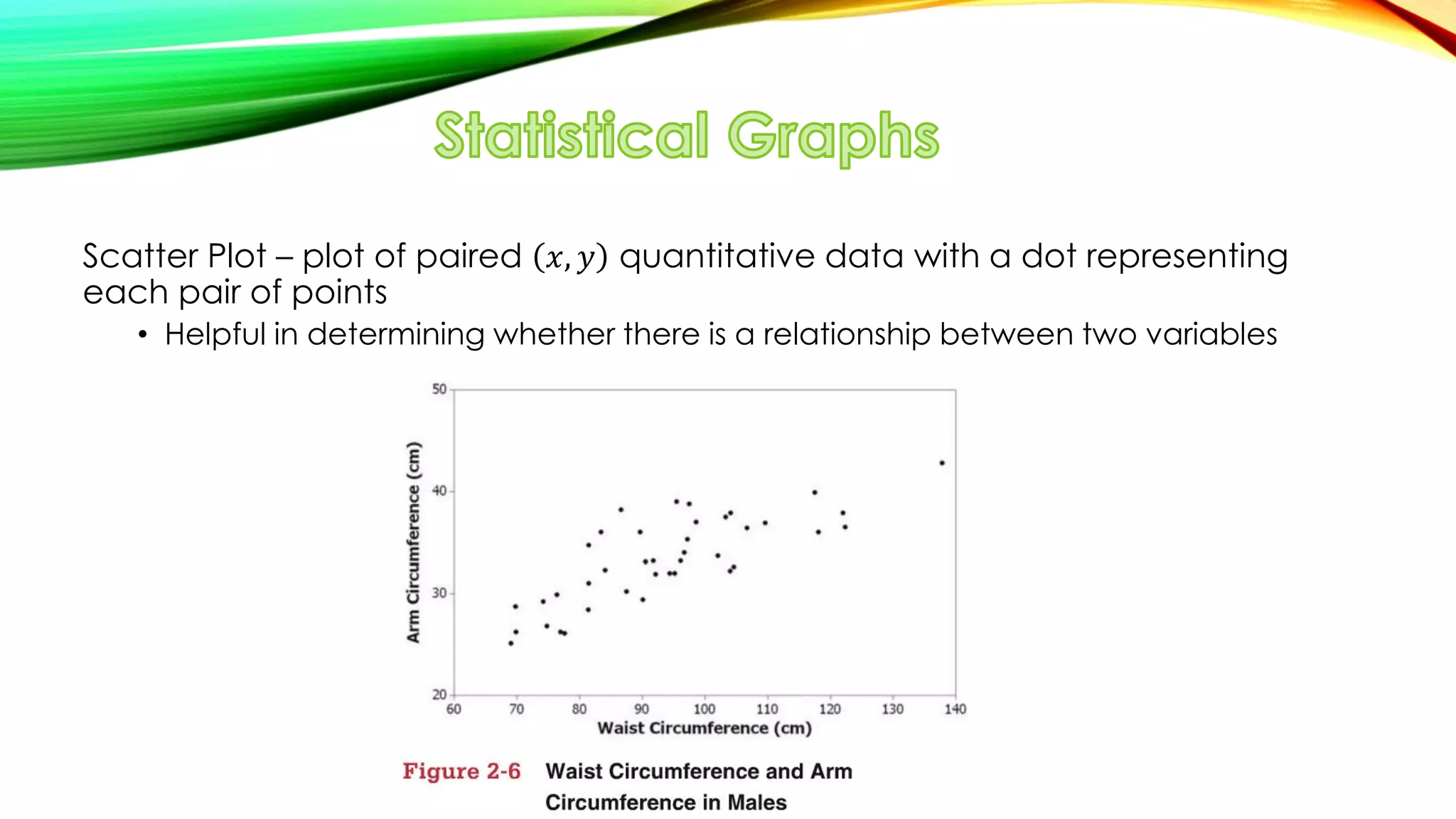
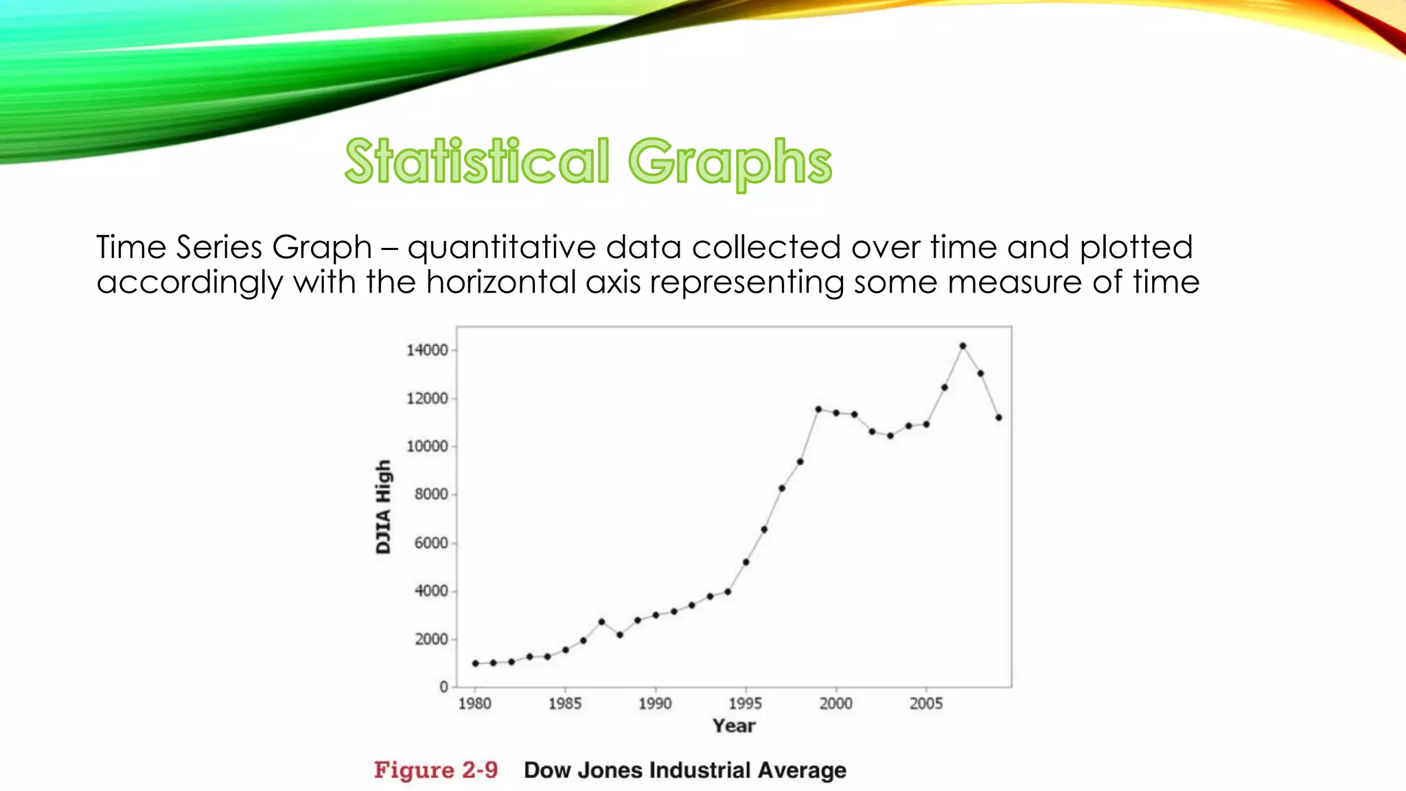


The document discusses simple linear regression. It defines key terms like regression equation, regression line, slope, intercept, residuals, and residual plot. It provides examples of using sample data to generate a regression equation and evaluating that regression model. Specifically, it shows generating a regression equation from bivariate data, checking assumptions visually through scatter plots and residual plots, and interpreting the slope as the marginal change in the response variable from a one unit change in the explanatory variable.