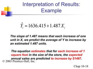
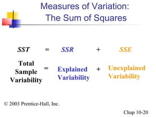
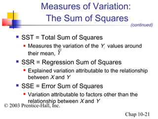
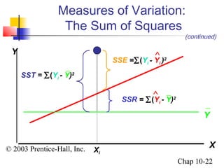
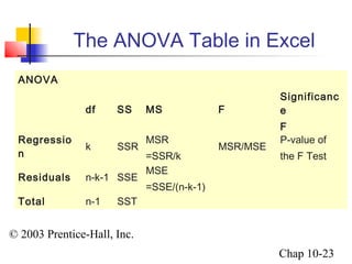
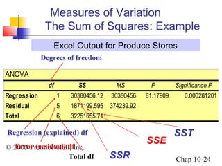
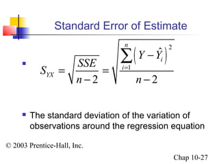
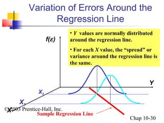
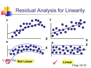
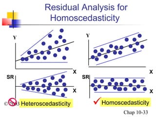
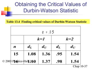
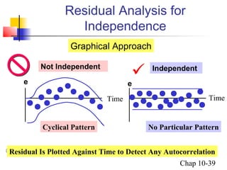
Business Statistics: 
A First Course 
(3rd Edition) 
Chapter 10 
Simple Linear Regression 
© 2003 Prentice-Hall, Inc. Chap 10-1
© 2003 Prentice-Hall, Inc. 
Chap 10-2 
Chapter Topics 
 Types of Regression Models 
 Determining the Simple Linear Regression 
Equation 
 Measures of Variation 
 Assumptions of Regression and Correlation 
 Residual Analysis 
 Measuring Autocorrelation 
 Inferences about the Slope
© 2003 Prentice-Hall, Inc. 
(continued) 
Chap 10-3 
Chapter Topics 
 Correlation - Measuring the Strength of the 
Association 
 Estimation of Mean Values and Prediction of 
Individual Values 
 Pitfalls in Regression and Ethical Issues
Purpose of Regression Analysis 
 Regression Analysis is Used Primarily to 
Model Causality and Provide Prediction 
 Predict the values of a dependent (response) 
variable based on values of at least one 
independent (explanatory) variable 
 Explain the effect of the independent variables on 
the dependent variable 
© 2003 Prentice-Hall, Inc. 
Chap 10-4
Types of Regression Models 
© 2003 Prentice-Hall, Inc. 
Chap 10-5 
Positive Linear Relationship 
Negative Linear Relationship 
Relationship NOT Linear 
No Relationship
Simple Linear Regression Model 
 Relationship Between Variables is Described 
by a Linear Function 
 The Change of One Variable Causes the 
Other Variable to Change 
 A Dependency of One Variable on the Other 
© 2003 Prentice-Hall, Inc. 
Chap 10-6
Simple Linear Regression Model 
Population regression line is a straight line that 
describes the dependence of the aavveerraaggee vvaalluuee 
((ccoonnddiittiioonnaall mmeeaann)) of one variable on the other 
Population 
Y intercept 
i i i Y b b X e 0 1 = + + 
© 2003 Prentice-Hall, Inc. 
Chap 10-7 
Population 
Regression 
Line 
(conditional mean) 
Population 
Slope 
Coefficient 
Random 
Error 
Dependent 
(Response) 
Variable 
Independent 
(Explanatory) 
Variable 
Y|X m 
(continued)
Simple Linear Regression Model 
© 2003 Prentice-Hall, Inc. 
(continued) 
i i i Y b b X e 0 1 = + + 
Chap 10-8 
= Random Error 
Y 
X 
(Observed Value of Y) = 
Observed Value of Y 
Y|X i m b b X 0 1 = + 
i e 
b0 
b1 
(Conditional Mean)
Linear Regression Equation 
Sample regression line provides an eessttiimmaattee 
of the population regression line as well as a 
predicted value of Y 
Yˆ =b +b X = Simple Regression Equation 
© 2003 Prentice-Hall, Inc. 
Chap 10-9 
Sample 
Y Intercept 
Sample 
Slope 
Coefficient 
i 0 1 i i Residual Y = b + b X + e 
0 1 
(Fitted Regression Line, Predicted Value)
Linear Regression Equation 
0 b 1 b 
 and are obtained by finding the values of 
0 b 1 b 
and that minimizes the sum of the 
ˆ n n 
å - =å 
Y Y e 
0 b b0 
1 b b1 
© 2003 Prentice-Hall, Inc. 
Chap 10-10 
squared residuals 
 provides an eessttiimmaattee of 
 provides and eessttiimmaattee of 
(continued) 
( )2 2 
i i i 
1 1 
i i 
= =
Linear Regression Equation 
i 0 1 i i Y = b + b X + e 
© 2003 Prentice-Hall, Inc. 
(continued) 
i i i Y b b X e 0 1 = + + 
Chap 10-11 
Y 
X 
Observed Value 
Y|X i m b b X 0 1 = + 
i e 
b0 
b1 
Y ˆ= b + b X 
i 0 1 
i i e 
1 b 
0 b
Interpretation of the Slope and 
Y |X 0 b m 0 = = 
| 
m 
© 2003 Prentice-Hall, Inc. 
Chap 10-12 
Intercept 
 is the average value of Y when 
the value of X is zero. 
 1 
measures the change in the 
average value of Y as a result of a one-unit 
change in X. 
Y X 
X 
b 
D 
= 
D
Interpretation of the Slope and 
| 0 ˆY X b m 0 = = 
Dm 
ˆb = 
Y | 
X 
© 2003 Prentice-Hall, Inc. 
(continued) 
Chap 10-13 
Intercept 
 is the eessttiimmaatteedd average value of 
Y when the value of X is zero. 
 1 
D 
X 
is the eessttiimmaatteedd change in the 
average value of Y as a result of a one-unit 
change in X.
Simple Linear Regression: 
© 2003 Prentice-Hall, Inc. 
Chap 10-14 
Example 
You wish to examine 
the linear dependency 
of the annual sales of 
produce stores on their 
sizes in square 
footage. Sample data 
for 7 stores were 
obtained. Find the 
equation of the straight 
line that fits the data 
best. 
Annual 
Store Square Sales 
Feet ($1000) 
1 1,726 3,681 
2 1,542 3,395 
3 2,816 6,653 
4 5,555 9,543 
5 1,292 3,318 
6 2,208 5,563 
7 1,313 3,760
Scatter Diagram: Example 
12000 
10000 
8000 
6000 
4000 
2000 
© 2003 Prentice-Hall, Inc. 
Chap 10-15 
0 
0 1000 2000 3000 4000 5000 6000 
Square Feet 
Annual Sales ($000) 
Excel Output
Simple Linear Regression 
ˆ 
i i 
1636.415 1.487 
© 2003 Prentice-Hall, Inc. 
Chap 10-16 
Equation: Example 
0 1 
i 
Y b b X 
X 
= + 
= + 
From Excel Printout: 
Coefficients 
Intercept 1636.414726 
X Variable 1 1.486633657
Graph of the Simple Linear 
Regression Equation: Example 
12000 
10000 
8000 
6000 
4000 
2000 
© 2003 Prentice-Hall, Inc. 
Chap 10-17 
0 
0 1000 2000 3000 4000 5000 6000 
Square Feet 
Annual Sales ($000) 
Yi = 1636.415 +1.487Xi 
Ù
Interpretation of Results: 
Yˆi = 1636.415 +1.487Xi 
© 2003 Prentice-Hall, Inc. 
Chap 10-18 
Example 
The slope of 1.487 means that each increase of one 
unit in X, we predict the average of Y to increase by 
an estimated 1.487 units. 
The equation estimates that for each increase of 1 
square foot in the size of the store, the expected 
annual sales are predicted to increase by $1487.
Simple Linear Regression in 
© 2003 Prentice-Hall, Inc. 
Chap 10-19 
PHStat 
 In Excel, use PHStat | Regression | Simple 
Linear Regression … 
 EXCEL Spreadsheet of Regression Sales on 
Footage 
Microsoft Excel 
Worksheet
Measures of Variation: 
The Sum of Squares 
SST = SSR + SSE 
Total 
Sample 
Variability 
© 2003 Prentice-Hall, Inc. 
Chap 10-20 
= Explained 
Variability 
+ Unexplained 
Variability
Measures of Variation: 
The Sum of Squares 
Y 
© 2003 Prentice-Hall, Inc. 
(continued) 
Chap 10-21 
 SST = Total Sum of Squares 
 Measures the variation of the Yi 
values around 
their mean, 
 SSR = Regression Sum of Squares 
 Explained variation attributable to the relationship 
between X and Y 
 SSE = Error Sum of Squares 
 Variation attributable to factors other than the 
relationship between X and Y
Measures of Variation: 
The Sum of Squares 
© 2003 Prentice-Hall, Inc. 
(continued) 
Chap 10-22 
Xi 
Y 
X 
Y 
SST = å(Yi - Y)2 
Ù 
SSE =å(Yi - Yi )2 
Ù 
SSR = å(Yi - Y)2 
_ 
_ 
_
The ANOVA Table in Excel 
© 2003 Prentice-Hall, Inc. 
Chap 10-23 
ANOVA 
df SS MS F 
Significanc 
e 
F 
Regressio 
n k SSR MSR 
=SSR/k 
MSR/MSE P-value of 
the F Test 
Residuals n-k-1 SSE MSE 
=SSE/(n-k-1) 
Total n-1 SST
Measures of Variation 
The Sum of Squares: Example 
Excel Output for Produce Stores 
Degrees of freedom 
© 2003 Prentice-Hall, Inc. 
Chap 10-24 
ANOVA 
df SS MS F Significance F 
Regression 1 30380456.12 30380456 81.17909 0.000281201 
Residual 5 1871199.595 374239.92 
Total 6 32251655.71 
SSR 
SSE 
Regression (explained) df 
Error (residual) df 
Total df 
SST
The Coefficient of Determination 
r SSR 
2 Regression Sum of Squares 
= = 
SST 
© 2003 Prentice-Hall, Inc. 
Total Sum of Squares 
Chap 10-25 
 
 Measures the proportion of variation in Y that 
is explained by the independent variable X in 
the regression model
Coefficients of Determination (r 2) 
r = +1 r = -1 
^ 
^ 
r = +0.9 r = 0 
© 2003 Prentice-Hall, Inc. 
Chap 10-26 
and Correlation (r) 
r2 = 1, r2 = 1, 
r2 = .81, Y r2 = 0, 
^ 
Yi = b0 + b1XiX 
Y 
Yi = b0 + b1Xi 
X 
^ 
Y 
Yi = b0 + b1XiX 
Y 
Yi = b0 + b1XiX
Standard Error of Estimate 
S SSE 
YX 
å 
= 
= = 
n n 
© 2003 Prentice-Hall, Inc. 
Chap 10-27 
 
n 
( ˆ 
)2 
1 
i 
Y - 
Y 
- - 
2 2 
i 
 The standard deviation of the variation of 
observations around the regression equation
Measures of Variation: 
Produce Store Example 
Excel Output for Produce Stores 
© 2003 Prentice-Hall, Inc. 
Chap 10-28 
Regression Statistics 
Multiple R 0.9705572 
R Square 0.94198129 
Adjusted R Square 0.93037754 
Standard Error 611.751517 
Observations 7 
r2 = .94 
94% of the variation in annual sales can be 
explained by the variability in the size of the 
store as measured by square footage 
Syx
Linear Regression Assumptions 
© 2003 Prentice-Hall, Inc. 
Chap 10-29 
 Normality 
 Y values are normally distributed for each X 
 Probability distribution of error is normal 
 2. Homoscedasticity (Constant Variance) 
 3. Independence of Errors
Variation of Errors Around the 
© 2003 Prentice-Hall, Inc. 
• Y values are normally distributed 
around the regression line. 
• For each X value, the “spread” or 
variance around the regression line is 
the same. 
Chap 10-30 
Regression Line 
X1 
X2 
X 
Y 
f(e ) 
Sample Regression Line
© 2003 Prentice-Hall, Inc. 
Chap 10-31 
Residual Analysis 
 Purposes 
 Examine linearity 
 Evaluate violations of assumptions 
 Graphical Analysis of Residuals 
 Plot residuals vs. X and time
Residual Analysis for Linearity 
e e 
© 2003 Prentice-Hall, Inc. 
Chap 10-32 
X 
Not Linear  Linear 
X 
Y 
X 
Y 
X
Residual Analysis for 
Homoscedasticity 
Y 
Heteroscedasticity Homoscedasticity 
© 2003 Prentice-Hall, Inc. 
Chap 10-33 
SR 
X 
SR 
X 
Y 
X X
Residual Analysis:Excel Output 
for Produce Stores Example 
Excel Output 
© 2003 Prentice-Hall, Inc. 
Chap 10-34 
Residual Plot 
0 1000 2000 3000 4000 5000 6000 
Square Feet 
Observation Predicted Y Residuals 
1 4202.344417 -521.3444173 
2 3928.803824 -533.8038245 
3 5822.775103 830.2248971 
4 9894.664688 -351.6646882 
5 3557.14541 -239.1454103 
6 4918.90184 644.0981603 
7 3588.364717 171.6352829
Residual Analysis for 
e e 
( ) 
© 2003 Prentice-Hall, Inc. 
Chap 10-35 
Independence 
 The Durbin-Watson Statistic 
 Used when data is collected over time to detect 
autocorrelation (residuals in one time period are 
related to residuals in another period) 
 Measures violation of independence assumption 
2 
1 
2 
2 
1 
n 
i i 
i 
n 
i 
i 
D 
e 
- 
= 
= 
- 
= 
å 
å 
Should be close to 2. 
If not, examine the model 
for autocorrelation.
Durbin-Watson Statistic in 
© 2003 Prentice-Hall, Inc. 
Chap 10-36 
PHStat 
 PHStat | Regression | Simple Linear 
Regression … 
 Check the box for Durbin-Watson Statistic
Obtaining the Critical Values of 
Durbin-Watson Statistic 
Table 13.4 Finding critical values of Durbin-Watson Statistic 
n dL dU dL dU 
15 1.08 1.36 .95 1.54 
16 1.10 1.37 .98 1.54 
© 2003 Prentice-Hall, Inc. 
a = .0 5 
k=1 k=2 
Chap 10-37
Using the Durbin-Watson 
: No autocorrelation (error terms are independent) 
: There is autocorrelation (error terms are not 
independent) 
Reject H0 
(positive 
autocorrelation) 
© 2003 Prentice-Hall, Inc. 
Inconclusive Reject H0 
(negative 
autocorrelation) 
Chap 10-38 
Statistic 
Accept H0 
(no autocorrelatin) 
0 H 
1 H 
0 d 2 4 L 4-dL dU 4-dU
Residual Analysis for 
Graphical Approach 
Cyclical Pattern No Particular Pattern 
© 2003 Prentice-Hall, Inc. 
Chap 10-39 
Independence 
Not Independent  Independent e e 
Time Time 
Residual Is Plotted Against Time to Detect Any Autocorrelation
Inference about the Slope: 
t b S S 
1 1 
© 2003 Prentice-Hall, Inc. 
Chap 10-40 
t Test 
 t Test for a Population Slope 
 Is there a linear dependency of Y on X ? 
 Null and Alternative Hypotheses 
 H0: b1 = 0 (No Linear Dependency) 
 H1: b1 ¹ 0 (Linear Dependency) 
 Test Statistic 
 
 
1 
1 
2 
1 
where 
YX 
( ) 
b n 
b 
i 
i 
S 
X X 
b 
= 
= - = 
å - 
d. f . = n - 2
Example: Produce Store 
© 2003 Prentice-Hall, Inc. 
Chap 10-41 
Data for 7 Stores: 
Estimated Regression 
Equation: 
The slope of this 
model is 1.487. 
Does Square 
Footage Affect 
Annual Sales? 
Annual 
Store Square Sales 
Feet ($000) 
1 1,726 3,681 
2 1,542 3,395 
3 2,816 6,653 
4 5,555 9,543 
5 1,292 3,318 
6 2,208 5,563 
7 1,313 3,760 
Yˆ =1636.415 +1.487Xi
Inferences about the Slope: 
: b1 ¹ 0 
a = .05 
df = 7 - 2 = 5 
Critical Value(s): 
From Excel Printout 
1 b b1 S t 
Intercept 1636.4147 451.4953 3.6244 0.01515 
Footage 1.4866 0.1650 9.0099 0.00028 
Reject Reject 
.025 
.025 
© 2003 Prentice-Hall, Inc. 
Coefficients Standard Error t Stat P-value 
Chap 10-42 
t Test Example 
H0: b1 = 0 
H1 
Test Statistic: 
Decision: 
Conclusion: 
There is evidence that 
square footage affects 
annual sales. 
-2.5706 0 2.5706 t 
Reject H0
Inferences about the Slope: 
Confidence Interval Example 
Confidence Interval Estimate of the Slope: 
Intercept 475.810926 2797.01853 
X Variable 11.06249037 1.91077694 
© 2003 Prentice-Hall, Inc. 
Chap 10-43 
1 n 2 b1 b t S - ± 
Excel Printout for Produce Stores 
Lower 95% Upper 95% 
At 95% level of confidence the confidence interval 
for the slope is (1.062, 1.911). Does not include 0. 
Conclusion: There is a significant linear dependency 
of annual sales on the size of the store.
Inferences about the Slope: 
SSR 
1 
2 
F SSE 
( n 
) 
= 
- 
© 2003 Prentice-Hall, Inc. 
Chap 10-44 
F Test 
 F Test for a Population Slope 
 Is there a linear dependency of Y on X ? 
 Null and Alternative Hypotheses 
 H0: b1 = 0 (No Linear Dependency) 
 H1: b1 ¹ 0 (Linear Dependency) 
 Test Statistic 
 
 Numerator d.f.=1, denominator d.f.=n-2
Relationship between a t Test 
© 2003 Prentice-Hall, Inc. 
Chap 10-45 
and an F Test 
 Null and Alternative Hypotheses 
 H: b= 0 (No Linear Dependency) 
01  H1: b1 ¹ 0 (Linear Dependency) 
( t )2 
= 
F n - 2 1,n - 2
Inferences about the Slope: 
F Test Example 
Reject 
© 2003 Prentice-Hall, Inc. 
From Excel Printout 
Reject H0 
Chap 10-46 
ANOVA 
Test Statistic: 
df SS MS F Significance F 
Regression 1 30380456.12 30380456.12 81.179 0.000281 
Residual 5 1871199.595 374239.919 
Total 6 32251655.71 
Decision: 
Conclusion: 
H0: b1 = 0 
H1: b1 ¹ 0 
a = .05 
numerator 
df = 1 
denominator 
df = 7 - 2 = 5 
There is evidence that 
square footage affects 
annual sales. 
0 6.61 
a = .05 
1,n 2 F -
Purpose of Correlation Analysis 
 Correlation Analysis is Used to Measure 
Strength of Association (Linear Relationship) 
Between 2 Numerical Variables 
 Only Strength of the Relationship is Concerned 
 No Causal Effect is Implied 
© 2003 Prentice-Hall, Inc. 
Chap 10-47
Purpose of Correlation Analysis 
(continued) 
 Population Correlation Coefficient r (Rho) is 
Used to Measure the Strength between the 
Variables 
 Sample Correlation Coefficient r is an 
Estimate of r  and is Used to Measure the 
Strength of the Linear Relationship in the 
Sample Observations 
© 2003 Prentice-Hall, Inc. 
Chap 10-48
Sample of Observations from 
Various r Values 
r = -1 r = -.6 r = 0 
© 2003 Prentice-Hall, Inc. 
r = .6 r = 1 Chap 10-49 
Y 
X 
Y 
X 
Y 
X 
Y 
X 
Y 
X
Features of r and r 
 Unit Free 
 Range between -1 and 1 
 The Closer to -1, the Stronger the Negative 
Linear Relationship 
 The Closer to 1, the Stronger the Positive 
Linear Relationship 
 The Closer to 0, the Weaker the Linear 
Relationship 
© 2003 Prentice-Hall, Inc. 
Chap 10-50
t Test for Correlation 
© 2003 Prentice-Hall, Inc. 
Chap 10-51 
 Hypotheses 
 H0: r = 0 (No Correlation) 
 H1: r ¹ 0 (Correlation) 
 Test Statistic 
 
where 
( ) ( ) 
( ) ( ) 
2 
å 
å å 
2 1 
2 2 
1 1 
2 
n 
i i 
i 
n n 
i i 
i i 
t r 
r 
n 
X X Y Y 
r r 
X X Y Y 
r 
= 
= = 
= - 
1 - 
- 
- - 
= = 
- -
Example: Produce Stores 
Is there any 
evidence of linear 
relationship between 
Annual Sales of a 
store and its Square 
Footage at .05 level 
of significance? H0: r = 0 (No association) 
© 2003 Prentice-Hall, Inc. 
From Excel Printout r 
Regression Statistics 
Multiple R 0.9705572 
R Square 0.94198129 
Adjusted R Square 0.93037754 
Standard Error 611.751517 
Observations 7 
H1: r ¹ 0 (Association) 
a = .05 
df = 7 - 2 = 5 
Chap 10-52
Example: Produce Stores 
= - r = = 
1- - 
- 
Critical Value(s): 
Reject Reject 
.025 
.025 
© 2003 Prentice-Hall, Inc. 
Chap 10-53 
Solution 
-2.5706 0 2.5706 
Decision: 
Reject H0 
Conclusion: 
There is evidence of a 
linear relationship at 5% 
level of significance 
2 
.9706 9.0099 
1 .9420 
2 5 
t r 
r 
n 
The value of the t statistic is 
exactly the same as the t 
statistic value for test on the 
slope coefficient
Estimation of Mean Values 
Confidence Interval Estimate for : 
The Mean of Y given a particular Xi 
Y ± t S + X - 
X 
Y|X Xi m = 
ˆ 1 ( ) 
å - t value from table 
with df=n-2 
© 2003 Prentice-Hall, Inc. 
2 
Chap 10-54 
2 
2 
n X X 
1 
i 
( ) 
i n YX n 
i 
i 
- 
= 
Standard error 
of the estimate 
Size of interval vary according to 
distance away from mean, X
Prediction of Individual Values 
Prediction Interval for Individual 
Y ± t S + + X - 
X 
ˆ 1 1 ( ) 
© 2003 Prentice-Hall, Inc. 
Chap 10-55 
Response Yi at a Particular Xi 
Addition of 1 increases width of interval 
from that for the mean of Y 
2 
2 
2 
n X X 
å - 
1 
i 
( ) 
i n YX n 
i 
i 
- 
=
Interval Estimates for Different 
© 2003 Prentice-Hall, Inc. 
Confidence 
Interval for the 
mean of Y 
Chap 10-56 
Values of X 
Y 
X 
Prediction Interval 
for a individual Yi 
A given X 
Yi = b0 + b1Xi 
Ù 
X
Example: Produce Stores 
© 2003 Prentice-Hall, Inc. 
Consider a store 
with 2000 square 
feet. 
Chap 10-57 
Data for 7 Stores: 
Regression Equation 
Obtained: 
Annual 
Store Square Sales 
Feet ($000) 
1 1,726 3,681 
2 1,542 3,395 
3 2,816 6,653 
4 5,555 9,543 
5 1,292 3,318 
6 2,208 5,563 
7 1,313 3,760 
Yˆ =1636.415 +1.487Xi
Estimation of Mean Values: 
Confidence Interval Estimate for Y|X Xi m = 
Y t S X X 
± + - = ± 
ˆ 1 ( ) 4610.45 612.66 
n X X 
å - 
© 2003 Prentice-Hall, Inc. 
Chap 10-58 
Example 
Find the 95% confidence interval for the average annual 
sales for stores of 2,000 square feet 
2 
2 
2 
1 
i 
( ) 
i n YX n 
i 
i 
- 
= 
Predicted Sales 
ˆ 1636.415 1.487 4610.45( $000) i Y = + X = 
2 5 2350.29 611.75 2.5706 YX n X S t t - = = = =
Prediction Interval for Y : 
Prediction Interval for Individual 
Y t S X X 
± + + - = ± 
ˆ 1 1 ( ) 4610.45 1687.68 
n X X 
© 2003 Prentice-Hall, Inc. 
Chap 10-59 
Example 
Find the 95% prediction interval for annual sales of one 
particular store of 2,000 square feet 
Predicted Sales) 
2 
2 
2 
å - 
1 
i 
( ) 
i n YX n 
i 
i 
- 
= 
X Xi Y = 
ˆ 1636.415 1.487 4610.45( $000) i Y = + X = 
2 5 2350.29 611.75 2.5706 YX n X S t t - = = = =
Estimation of Mean Values and 
Prediction of Individual Values in PHStat 
 In Excel, use PHStat | Regression | Simple 
Linear Regression … 
 Check the “Confidence and Prediction Interval for 
X=” box 
 EXCEL Spreadsheet of Regression Sales on 
Footage 
© 2003 Prentice-Hall, Inc. 
Chap 10-60 
Microsoft Excel 
Worksheet
Pitfalls of Regression Analysis 
 Lacking an Awareness of the Assumptions 
Underlining Least-squares Regression 
 Not Knowing How to Evaluate the Assumptions 
 Not Knowing What the Alternatives to Least-squares 
© 2003 Prentice-Hall, Inc. 
Chap 10-61 
Regression are if a Particular 
Assumption is Violated 
 Using a Regression Model Without Knowledge 
of the Subject Matter
Strategy for Avoiding the Pitfalls 
© 2003 Prentice-Hall, Inc. 
Chap 10-62 
of Regression 
 Start with a scatter plot of X on Y to observe 
possible relationship 
 Perform residual analysis to check the 
assumptions 
 Use a histogram, stem-and-leaf display, box-and- 
whisker plot, or normal probability plot of 
the residuals to uncover possible non-normality
Strategy for Avoiding the Pitfalls 
© 2003 Prentice-Hall, Inc. 
(continued) 
Chap 10-63 
of Regression 
 If there is violation of any assumption, use 
alternative methods (e.g., least absolute 
deviation regression or least median of 
squares regression) to least-squares 
regression or alternative least-squares models 
(e.g., curvilinear or multiple regression) 
 If there is no evidence of assumption violation, 
then test for the significance of the regression 
coefficients and construct confidence intervals 
and prediction intervals
© 2003 Prentice-Hall, Inc. 
Chap 10-64 
Chapter Summary 
 Introduced Types of Regression Models 
 Discussed Determining the Simple Linear 
Regression Equation 
 Described Measures of Variation 
 Addressed Assumptions of Regression and 
Correlation 
 Discussed Residual Analysis 
 Addressed Measuring Autocorrelation
© 2003 Prentice-Hall, Inc. 
(continued) 
Chap 10-65 
Chapter Summary 
 Described Inference about the Slope 
 Discussed Correlation - Measuring the 
Strength of the Association 
 Addressed Estimation of Mean Values and 
Prediction of Individual Values 
 Discussed Pitfalls in Regression and Ethical 
Issues

Linear regression

  • 1.
    Business Statistics: AFirst Course (3rd Edition) Chapter 10 Simple Linear Regression © 2003 Prentice-Hall, Inc. Chap 10-1
  • 2.
    © 2003 Prentice-Hall,Inc. Chap 10-2 Chapter Topics  Types of Regression Models  Determining the Simple Linear Regression Equation  Measures of Variation  Assumptions of Regression and Correlation  Residual Analysis  Measuring Autocorrelation  Inferences about the Slope
  • 3.
    © 2003 Prentice-Hall,Inc. (continued) Chap 10-3 Chapter Topics  Correlation - Measuring the Strength of the Association  Estimation of Mean Values and Prediction of Individual Values  Pitfalls in Regression and Ethical Issues
  • 4.
    Purpose of RegressionAnalysis  Regression Analysis is Used Primarily to Model Causality and Provide Prediction  Predict the values of a dependent (response) variable based on values of at least one independent (explanatory) variable  Explain the effect of the independent variables on the dependent variable © 2003 Prentice-Hall, Inc. Chap 10-4
  • 5.
    Types of RegressionModels © 2003 Prentice-Hall, Inc. Chap 10-5 Positive Linear Relationship Negative Linear Relationship Relationship NOT Linear No Relationship
  • 6.
    Simple Linear RegressionModel  Relationship Between Variables is Described by a Linear Function  The Change of One Variable Causes the Other Variable to Change  A Dependency of One Variable on the Other © 2003 Prentice-Hall, Inc. Chap 10-6
  • 7.
    Simple Linear RegressionModel Population regression line is a straight line that describes the dependence of the aavveerraaggee vvaalluuee ((ccoonnddiittiioonnaall mmeeaann)) of one variable on the other Population Y intercept i i i Y b b X e 0 1 = + + © 2003 Prentice-Hall, Inc. Chap 10-7 Population Regression Line (conditional mean) Population Slope Coefficient Random Error Dependent (Response) Variable Independent (Explanatory) Variable Y|X m (continued)
  • 8.
    Simple Linear RegressionModel © 2003 Prentice-Hall, Inc. (continued) i i i Y b b X e 0 1 = + + Chap 10-8 = Random Error Y X (Observed Value of Y) = Observed Value of Y Y|X i m b b X 0 1 = + i e b0 b1 (Conditional Mean)
  • 9.
    Linear Regression Equation Sample regression line provides an eessttiimmaattee of the population regression line as well as a predicted value of Y Yˆ =b +b X = Simple Regression Equation © 2003 Prentice-Hall, Inc. Chap 10-9 Sample Y Intercept Sample Slope Coefficient i 0 1 i i Residual Y = b + b X + e 0 1 (Fitted Regression Line, Predicted Value)
  • 10.
    Linear Regression Equation 0 b 1 b  and are obtained by finding the values of 0 b 1 b and that minimizes the sum of the ˆ n n å - =å Y Y e 0 b b0 1 b b1 © 2003 Prentice-Hall, Inc. Chap 10-10 squared residuals  provides an eessttiimmaattee of  provides and eessttiimmaattee of (continued) ( )2 2 i i i 1 1 i i = =
  • 11.
    Linear Regression Equation i 0 1 i i Y = b + b X + e © 2003 Prentice-Hall, Inc. (continued) i i i Y b b X e 0 1 = + + Chap 10-11 Y X Observed Value Y|X i m b b X 0 1 = + i e b0 b1 Y ˆ= b + b X i 0 1 i i e 1 b 0 b
  • 12.
    Interpretation of theSlope and Y |X 0 b m 0 = = | m © 2003 Prentice-Hall, Inc. Chap 10-12 Intercept  is the average value of Y when the value of X is zero.  1 measures the change in the average value of Y as a result of a one-unit change in X. Y X X b D = D
  • 13.
    Interpretation of theSlope and | 0 ˆY X b m 0 = = Dm ˆb = Y | X © 2003 Prentice-Hall, Inc. (continued) Chap 10-13 Intercept  is the eessttiimmaatteedd average value of Y when the value of X is zero.  1 D X is the eessttiimmaatteedd change in the average value of Y as a result of a one-unit change in X.
  • 14.
    Simple Linear Regression: © 2003 Prentice-Hall, Inc. Chap 10-14 Example You wish to examine the linear dependency of the annual sales of produce stores on their sizes in square footage. Sample data for 7 stores were obtained. Find the equation of the straight line that fits the data best. Annual Store Square Sales Feet ($1000) 1 1,726 3,681 2 1,542 3,395 3 2,816 6,653 4 5,555 9,543 5 1,292 3,318 6 2,208 5,563 7 1,313 3,760
  • 15.
    Scatter Diagram: Example 12000 10000 8000 6000 4000 2000 © 2003 Prentice-Hall, Inc. Chap 10-15 0 0 1000 2000 3000 4000 5000 6000 Square Feet Annual Sales ($000) Excel Output
  • 16.
    Simple Linear Regression ˆ i i 1636.415 1.487 © 2003 Prentice-Hall, Inc. Chap 10-16 Equation: Example 0 1 i Y b b X X = + = + From Excel Printout: Coefficients Intercept 1636.414726 X Variable 1 1.486633657
  • 17.
    Graph of theSimple Linear Regression Equation: Example 12000 10000 8000 6000 4000 2000 © 2003 Prentice-Hall, Inc. Chap 10-17 0 0 1000 2000 3000 4000 5000 6000 Square Feet Annual Sales ($000) Yi = 1636.415 +1.487Xi Ù
  • 18.
    Interpretation of Results: Yˆi = 1636.415 +1.487Xi © 2003 Prentice-Hall, Inc. Chap 10-18 Example The slope of 1.487 means that each increase of one unit in X, we predict the average of Y to increase by an estimated 1.487 units. The equation estimates that for each increase of 1 square foot in the size of the store, the expected annual sales are predicted to increase by $1487.
  • 19.
    Simple Linear Regressionin © 2003 Prentice-Hall, Inc. Chap 10-19 PHStat  In Excel, use PHStat | Regression | Simple Linear Regression …  EXCEL Spreadsheet of Regression Sales on Footage Microsoft Excel Worksheet
  • 20.
    Measures of Variation: The Sum of Squares SST = SSR + SSE Total Sample Variability © 2003 Prentice-Hall, Inc. Chap 10-20 = Explained Variability + Unexplained Variability
  • 21.
    Measures of Variation: The Sum of Squares Y © 2003 Prentice-Hall, Inc. (continued) Chap 10-21  SST = Total Sum of Squares  Measures the variation of the Yi values around their mean,  SSR = Regression Sum of Squares  Explained variation attributable to the relationship between X and Y  SSE = Error Sum of Squares  Variation attributable to factors other than the relationship between X and Y
  • 22.
    Measures of Variation: The Sum of Squares © 2003 Prentice-Hall, Inc. (continued) Chap 10-22 Xi Y X Y SST = å(Yi - Y)2 Ù SSE =å(Yi - Yi )2 Ù SSR = å(Yi - Y)2 _ _ _
  • 23.
    The ANOVA Tablein Excel © 2003 Prentice-Hall, Inc. Chap 10-23 ANOVA df SS MS F Significanc e F Regressio n k SSR MSR =SSR/k MSR/MSE P-value of the F Test Residuals n-k-1 SSE MSE =SSE/(n-k-1) Total n-1 SST
  • 24.
    Measures of Variation The Sum of Squares: Example Excel Output for Produce Stores Degrees of freedom © 2003 Prentice-Hall, Inc. Chap 10-24 ANOVA df SS MS F Significance F Regression 1 30380456.12 30380456 81.17909 0.000281201 Residual 5 1871199.595 374239.92 Total 6 32251655.71 SSR SSE Regression (explained) df Error (residual) df Total df SST
  • 25.
    The Coefficient ofDetermination r SSR 2 Regression Sum of Squares = = SST © 2003 Prentice-Hall, Inc. Total Sum of Squares Chap 10-25   Measures the proportion of variation in Y that is explained by the independent variable X in the regression model
  • 26.
    Coefficients of Determination(r 2) r = +1 r = -1 ^ ^ r = +0.9 r = 0 © 2003 Prentice-Hall, Inc. Chap 10-26 and Correlation (r) r2 = 1, r2 = 1, r2 = .81, Y r2 = 0, ^ Yi = b0 + b1XiX Y Yi = b0 + b1Xi X ^ Y Yi = b0 + b1XiX Y Yi = b0 + b1XiX
  • 27.
    Standard Error ofEstimate S SSE YX å = = = n n © 2003 Prentice-Hall, Inc. Chap 10-27  n ( ˆ )2 1 i Y - Y - - 2 2 i  The standard deviation of the variation of observations around the regression equation
  • 28.
    Measures of Variation: Produce Store Example Excel Output for Produce Stores © 2003 Prentice-Hall, Inc. Chap 10-28 Regression Statistics Multiple R 0.9705572 R Square 0.94198129 Adjusted R Square 0.93037754 Standard Error 611.751517 Observations 7 r2 = .94 94% of the variation in annual sales can be explained by the variability in the size of the store as measured by square footage Syx
  • 29.
    Linear Regression Assumptions © 2003 Prentice-Hall, Inc. Chap 10-29  Normality  Y values are normally distributed for each X  Probability distribution of error is normal  2. Homoscedasticity (Constant Variance)  3. Independence of Errors
  • 30.
    Variation of ErrorsAround the © 2003 Prentice-Hall, Inc. • Y values are normally distributed around the regression line. • For each X value, the “spread” or variance around the regression line is the same. Chap 10-30 Regression Line X1 X2 X Y f(e ) Sample Regression Line
  • 31.
    © 2003 Prentice-Hall,Inc. Chap 10-31 Residual Analysis  Purposes  Examine linearity  Evaluate violations of assumptions  Graphical Analysis of Residuals  Plot residuals vs. X and time
  • 32.
    Residual Analysis forLinearity e e © 2003 Prentice-Hall, Inc. Chap 10-32 X Not Linear  Linear X Y X Y X
  • 33.
    Residual Analysis for Homoscedasticity Y Heteroscedasticity Homoscedasticity © 2003 Prentice-Hall, Inc. Chap 10-33 SR X SR X Y X X
  • 34.
    Residual Analysis:Excel Output for Produce Stores Example Excel Output © 2003 Prentice-Hall, Inc. Chap 10-34 Residual Plot 0 1000 2000 3000 4000 5000 6000 Square Feet Observation Predicted Y Residuals 1 4202.344417 -521.3444173 2 3928.803824 -533.8038245 3 5822.775103 830.2248971 4 9894.664688 -351.6646882 5 3557.14541 -239.1454103 6 4918.90184 644.0981603 7 3588.364717 171.6352829
  • 35.
    Residual Analysis for e e ( ) © 2003 Prentice-Hall, Inc. Chap 10-35 Independence  The Durbin-Watson Statistic  Used when data is collected over time to detect autocorrelation (residuals in one time period are related to residuals in another period)  Measures violation of independence assumption 2 1 2 2 1 n i i i n i i D e - = = - = å å Should be close to 2. If not, examine the model for autocorrelation.
  • 36.
    Durbin-Watson Statistic in © 2003 Prentice-Hall, Inc. Chap 10-36 PHStat  PHStat | Regression | Simple Linear Regression …  Check the box for Durbin-Watson Statistic
  • 37.
    Obtaining the CriticalValues of Durbin-Watson Statistic Table 13.4 Finding critical values of Durbin-Watson Statistic n dL dU dL dU 15 1.08 1.36 .95 1.54 16 1.10 1.37 .98 1.54 © 2003 Prentice-Hall, Inc. a = .0 5 k=1 k=2 Chap 10-37
  • 38.
    Using the Durbin-Watson : No autocorrelation (error terms are independent) : There is autocorrelation (error terms are not independent) Reject H0 (positive autocorrelation) © 2003 Prentice-Hall, Inc. Inconclusive Reject H0 (negative autocorrelation) Chap 10-38 Statistic Accept H0 (no autocorrelatin) 0 H 1 H 0 d 2 4 L 4-dL dU 4-dU
  • 39.
    Residual Analysis for Graphical Approach Cyclical Pattern No Particular Pattern © 2003 Prentice-Hall, Inc. Chap 10-39 Independence Not Independent  Independent e e Time Time Residual Is Plotted Against Time to Detect Any Autocorrelation
  • 40.
    Inference about theSlope: t b S S 1 1 © 2003 Prentice-Hall, Inc. Chap 10-40 t Test  t Test for a Population Slope  Is there a linear dependency of Y on X ?  Null and Alternative Hypotheses  H0: b1 = 0 (No Linear Dependency)  H1: b1 ¹ 0 (Linear Dependency)  Test Statistic   1 1 2 1 where YX ( ) b n b i i S X X b = = - = å - d. f . = n - 2
  • 41.
    Example: Produce Store © 2003 Prentice-Hall, Inc. Chap 10-41 Data for 7 Stores: Estimated Regression Equation: The slope of this model is 1.487. Does Square Footage Affect Annual Sales? Annual Store Square Sales Feet ($000) 1 1,726 3,681 2 1,542 3,395 3 2,816 6,653 4 5,555 9,543 5 1,292 3,318 6 2,208 5,563 7 1,313 3,760 Yˆ =1636.415 +1.487Xi
  • 42.
    Inferences about theSlope: : b1 ¹ 0 a = .05 df = 7 - 2 = 5 Critical Value(s): From Excel Printout 1 b b1 S t Intercept 1636.4147 451.4953 3.6244 0.01515 Footage 1.4866 0.1650 9.0099 0.00028 Reject Reject .025 .025 © 2003 Prentice-Hall, Inc. Coefficients Standard Error t Stat P-value Chap 10-42 t Test Example H0: b1 = 0 H1 Test Statistic: Decision: Conclusion: There is evidence that square footage affects annual sales. -2.5706 0 2.5706 t Reject H0
  • 43.
    Inferences about theSlope: Confidence Interval Example Confidence Interval Estimate of the Slope: Intercept 475.810926 2797.01853 X Variable 11.06249037 1.91077694 © 2003 Prentice-Hall, Inc. Chap 10-43 1 n 2 b1 b t S - ± Excel Printout for Produce Stores Lower 95% Upper 95% At 95% level of confidence the confidence interval for the slope is (1.062, 1.911). Does not include 0. Conclusion: There is a significant linear dependency of annual sales on the size of the store.
  • 44.
    Inferences about theSlope: SSR 1 2 F SSE ( n ) = - © 2003 Prentice-Hall, Inc. Chap 10-44 F Test  F Test for a Population Slope  Is there a linear dependency of Y on X ?  Null and Alternative Hypotheses  H0: b1 = 0 (No Linear Dependency)  H1: b1 ¹ 0 (Linear Dependency)  Test Statistic   Numerator d.f.=1, denominator d.f.=n-2
  • 45.
    Relationship between at Test © 2003 Prentice-Hall, Inc. Chap 10-45 and an F Test  Null and Alternative Hypotheses  H: b= 0 (No Linear Dependency) 01  H1: b1 ¹ 0 (Linear Dependency) ( t )2 = F n - 2 1,n - 2
  • 46.
    Inferences about theSlope: F Test Example Reject © 2003 Prentice-Hall, Inc. From Excel Printout Reject H0 Chap 10-46 ANOVA Test Statistic: df SS MS F Significance F Regression 1 30380456.12 30380456.12 81.179 0.000281 Residual 5 1871199.595 374239.919 Total 6 32251655.71 Decision: Conclusion: H0: b1 = 0 H1: b1 ¹ 0 a = .05 numerator df = 1 denominator df = 7 - 2 = 5 There is evidence that square footage affects annual sales. 0 6.61 a = .05 1,n 2 F -
  • 47.
    Purpose of CorrelationAnalysis  Correlation Analysis is Used to Measure Strength of Association (Linear Relationship) Between 2 Numerical Variables  Only Strength of the Relationship is Concerned  No Causal Effect is Implied © 2003 Prentice-Hall, Inc. Chap 10-47
  • 48.
    Purpose of CorrelationAnalysis (continued)  Population Correlation Coefficient r (Rho) is Used to Measure the Strength between the Variables  Sample Correlation Coefficient r is an Estimate of r and is Used to Measure the Strength of the Linear Relationship in the Sample Observations © 2003 Prentice-Hall, Inc. Chap 10-48
  • 49.
    Sample of Observationsfrom Various r Values r = -1 r = -.6 r = 0 © 2003 Prentice-Hall, Inc. r = .6 r = 1 Chap 10-49 Y X Y X Y X Y X Y X
  • 50.
    Features of rand r  Unit Free  Range between -1 and 1  The Closer to -1, the Stronger the Negative Linear Relationship  The Closer to 1, the Stronger the Positive Linear Relationship  The Closer to 0, the Weaker the Linear Relationship © 2003 Prentice-Hall, Inc. Chap 10-50
  • 51.
    t Test forCorrelation © 2003 Prentice-Hall, Inc. Chap 10-51  Hypotheses  H0: r = 0 (No Correlation)  H1: r ¹ 0 (Correlation)  Test Statistic  where ( ) ( ) ( ) ( ) 2 å å å 2 1 2 2 1 1 2 n i i i n n i i i i t r r n X X Y Y r r X X Y Y r = = = = - 1 - - - - = = - -
  • 52.
    Example: Produce Stores Is there any evidence of linear relationship between Annual Sales of a store and its Square Footage at .05 level of significance? H0: r = 0 (No association) © 2003 Prentice-Hall, Inc. From Excel Printout r Regression Statistics Multiple R 0.9705572 R Square 0.94198129 Adjusted R Square 0.93037754 Standard Error 611.751517 Observations 7 H1: r ¹ 0 (Association) a = .05 df = 7 - 2 = 5 Chap 10-52
  • 53.
    Example: Produce Stores = - r = = 1- - - Critical Value(s): Reject Reject .025 .025 © 2003 Prentice-Hall, Inc. Chap 10-53 Solution -2.5706 0 2.5706 Decision: Reject H0 Conclusion: There is evidence of a linear relationship at 5% level of significance 2 .9706 9.0099 1 .9420 2 5 t r r n The value of the t statistic is exactly the same as the t statistic value for test on the slope coefficient
  • 54.
    Estimation of MeanValues Confidence Interval Estimate for : The Mean of Y given a particular Xi Y ± t S + X - X Y|X Xi m = ˆ 1 ( ) å - t value from table with df=n-2 © 2003 Prentice-Hall, Inc. 2 Chap 10-54 2 2 n X X 1 i ( ) i n YX n i i - = Standard error of the estimate Size of interval vary according to distance away from mean, X
  • 55.
    Prediction of IndividualValues Prediction Interval for Individual Y ± t S + + X - X ˆ 1 1 ( ) © 2003 Prentice-Hall, Inc. Chap 10-55 Response Yi at a Particular Xi Addition of 1 increases width of interval from that for the mean of Y 2 2 2 n X X å - 1 i ( ) i n YX n i i - =
  • 56.
    Interval Estimates forDifferent © 2003 Prentice-Hall, Inc. Confidence Interval for the mean of Y Chap 10-56 Values of X Y X Prediction Interval for a individual Yi A given X Yi = b0 + b1Xi Ù X
  • 57.
    Example: Produce Stores © 2003 Prentice-Hall, Inc. Consider a store with 2000 square feet. Chap 10-57 Data for 7 Stores: Regression Equation Obtained: Annual Store Square Sales Feet ($000) 1 1,726 3,681 2 1,542 3,395 3 2,816 6,653 4 5,555 9,543 5 1,292 3,318 6 2,208 5,563 7 1,313 3,760 Yˆ =1636.415 +1.487Xi
  • 58.
    Estimation of MeanValues: Confidence Interval Estimate for Y|X Xi m = Y t S X X ± + - = ± ˆ 1 ( ) 4610.45 612.66 n X X å - © 2003 Prentice-Hall, Inc. Chap 10-58 Example Find the 95% confidence interval for the average annual sales for stores of 2,000 square feet 2 2 2 1 i ( ) i n YX n i i - = Predicted Sales ˆ 1636.415 1.487 4610.45( $000) i Y = + X = 2 5 2350.29 611.75 2.5706 YX n X S t t - = = = =
  • 59.
    Prediction Interval forY : Prediction Interval for Individual Y t S X X ± + + - = ± ˆ 1 1 ( ) 4610.45 1687.68 n X X © 2003 Prentice-Hall, Inc. Chap 10-59 Example Find the 95% prediction interval for annual sales of one particular store of 2,000 square feet Predicted Sales) 2 2 2 å - 1 i ( ) i n YX n i i - = X Xi Y = ˆ 1636.415 1.487 4610.45( $000) i Y = + X = 2 5 2350.29 611.75 2.5706 YX n X S t t - = = = =
  • 60.
    Estimation of MeanValues and Prediction of Individual Values in PHStat  In Excel, use PHStat | Regression | Simple Linear Regression …  Check the “Confidence and Prediction Interval for X=” box  EXCEL Spreadsheet of Regression Sales on Footage © 2003 Prentice-Hall, Inc. Chap 10-60 Microsoft Excel Worksheet
  • 61.
    Pitfalls of RegressionAnalysis  Lacking an Awareness of the Assumptions Underlining Least-squares Regression  Not Knowing How to Evaluate the Assumptions  Not Knowing What the Alternatives to Least-squares © 2003 Prentice-Hall, Inc. Chap 10-61 Regression are if a Particular Assumption is Violated  Using a Regression Model Without Knowledge of the Subject Matter
  • 62.
    Strategy for Avoidingthe Pitfalls © 2003 Prentice-Hall, Inc. Chap 10-62 of Regression  Start with a scatter plot of X on Y to observe possible relationship  Perform residual analysis to check the assumptions  Use a histogram, stem-and-leaf display, box-and- whisker plot, or normal probability plot of the residuals to uncover possible non-normality
  • 63.
    Strategy for Avoidingthe Pitfalls © 2003 Prentice-Hall, Inc. (continued) Chap 10-63 of Regression  If there is violation of any assumption, use alternative methods (e.g., least absolute deviation regression or least median of squares regression) to least-squares regression or alternative least-squares models (e.g., curvilinear or multiple regression)  If there is no evidence of assumption violation, then test for the significance of the regression coefficients and construct confidence intervals and prediction intervals
  • 64.
    © 2003 Prentice-Hall,Inc. Chap 10-64 Chapter Summary  Introduced Types of Regression Models  Discussed Determining the Simple Linear Regression Equation  Described Measures of Variation  Addressed Assumptions of Regression and Correlation  Discussed Residual Analysis  Addressed Measuring Autocorrelation
  • 65.
    © 2003 Prentice-Hall,Inc. (continued) Chap 10-65 Chapter Summary  Described Inference about the Slope  Discussed Correlation - Measuring the Strength of the Association  Addressed Estimation of Mean Values and Prediction of Individual Values  Discussed Pitfalls in Regression and Ethical Issues