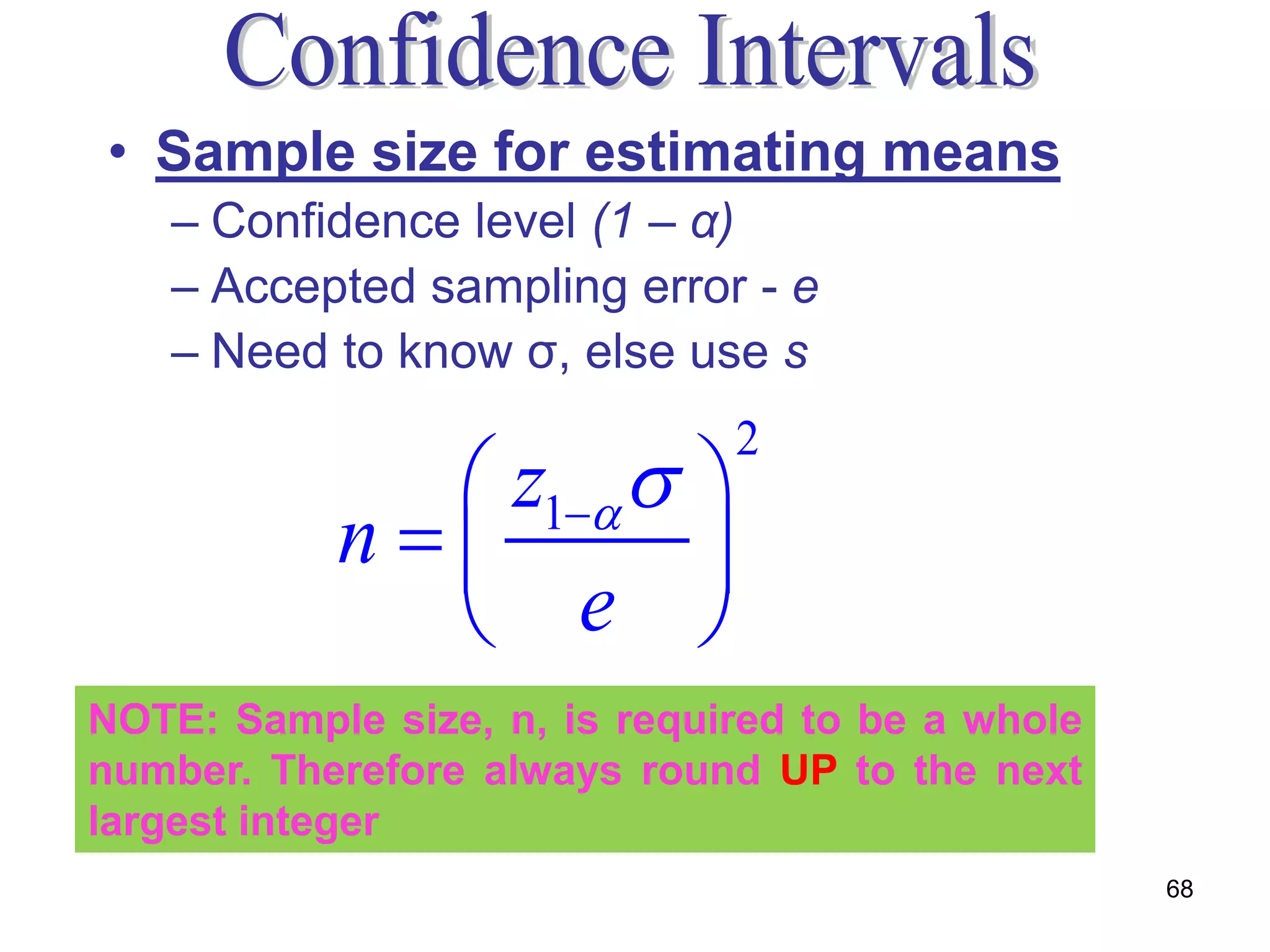
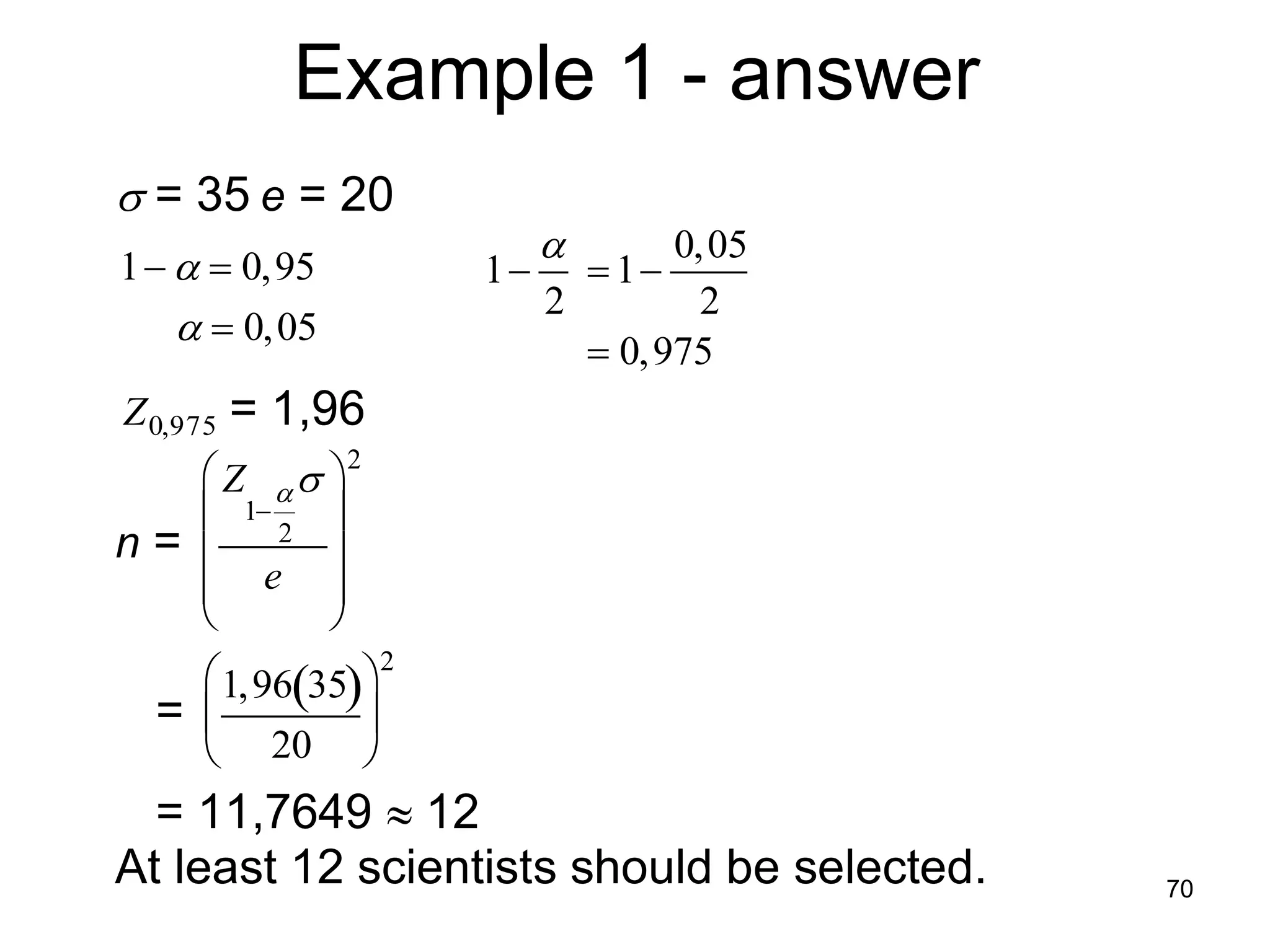
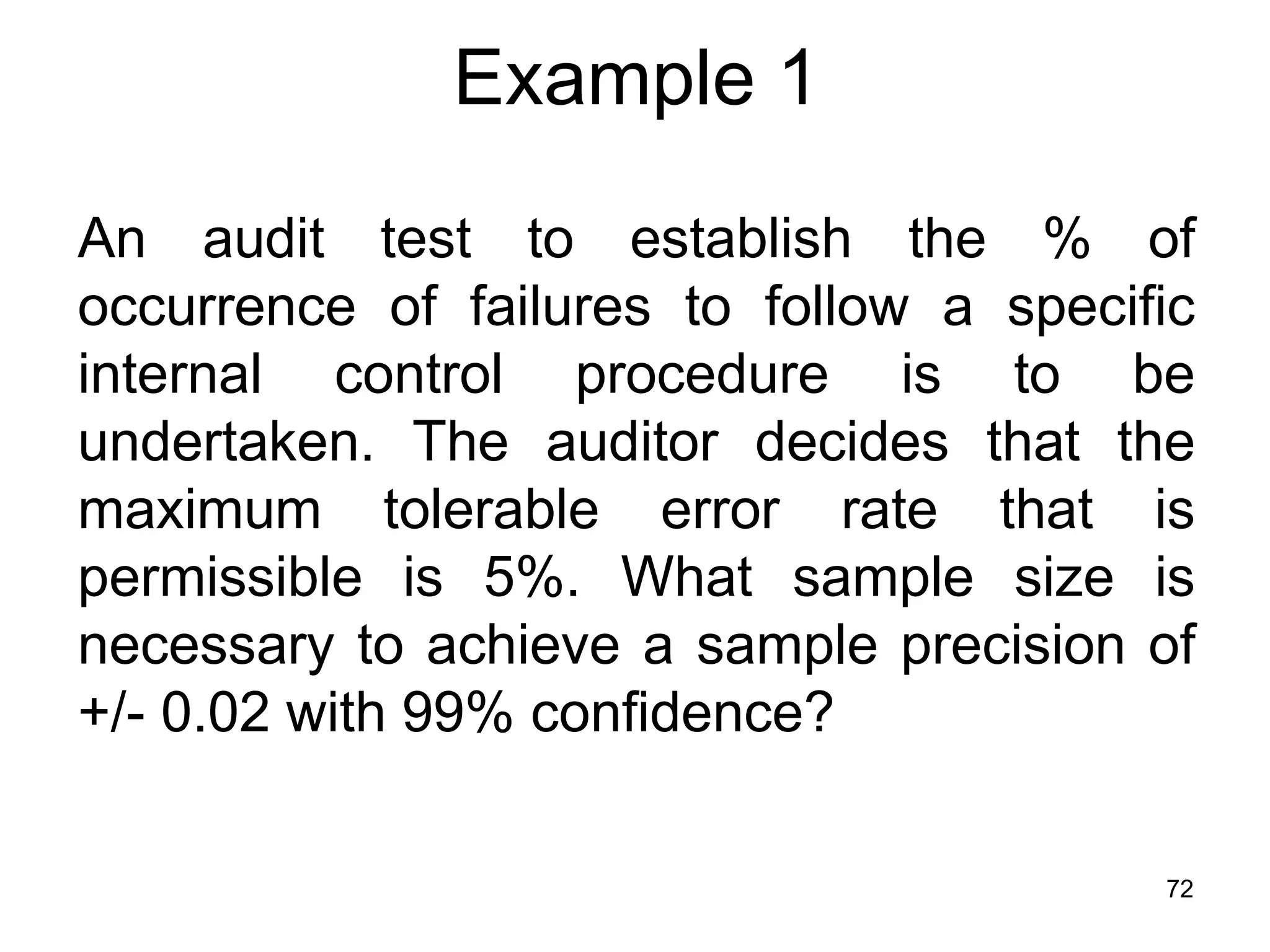
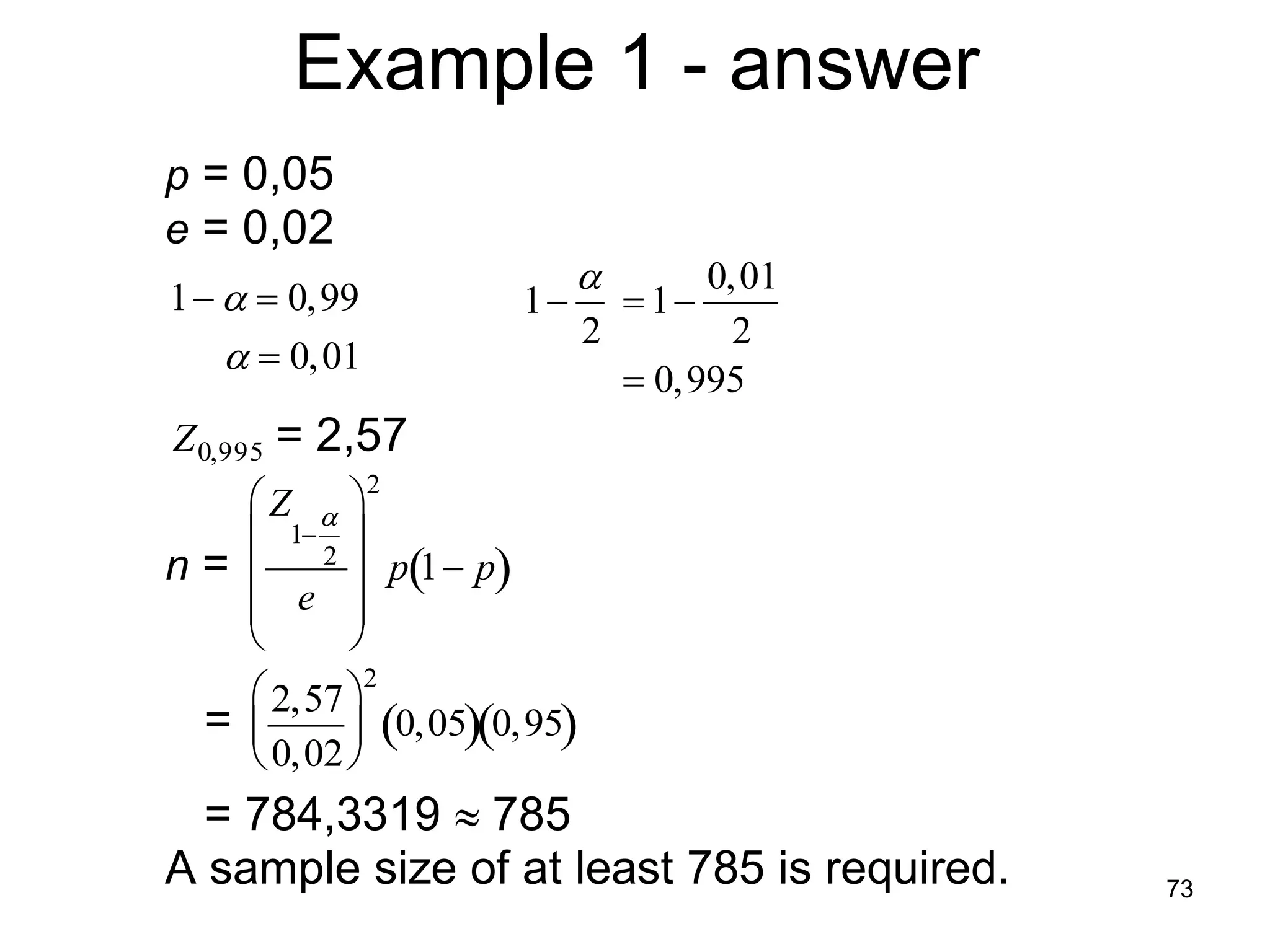
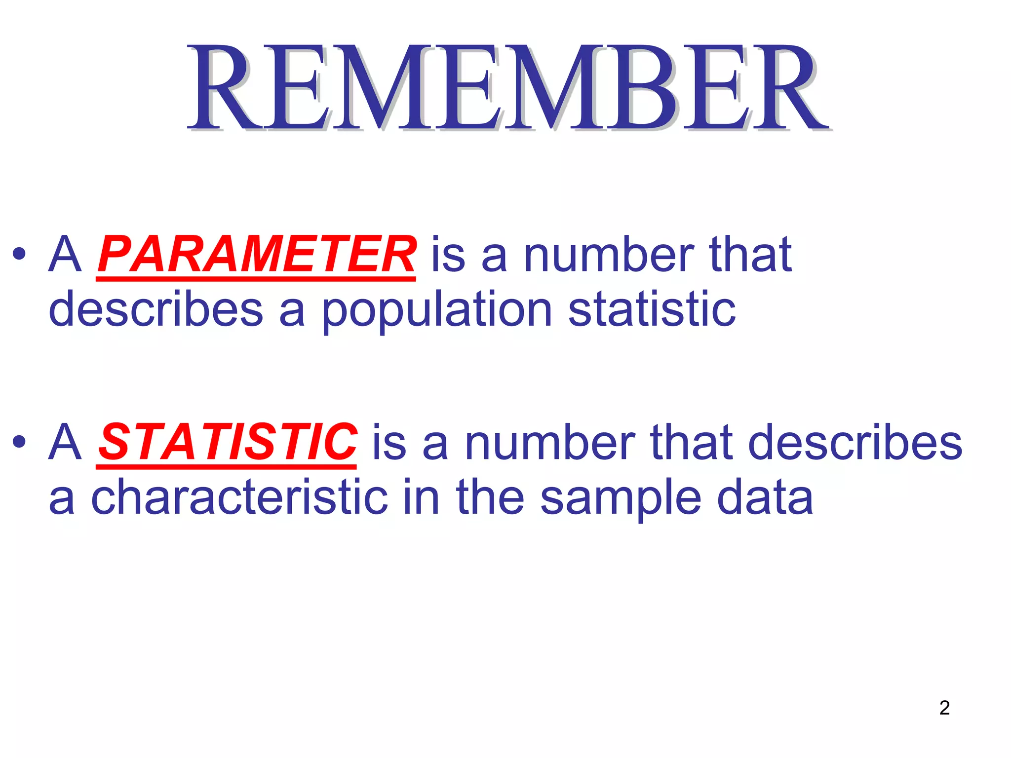
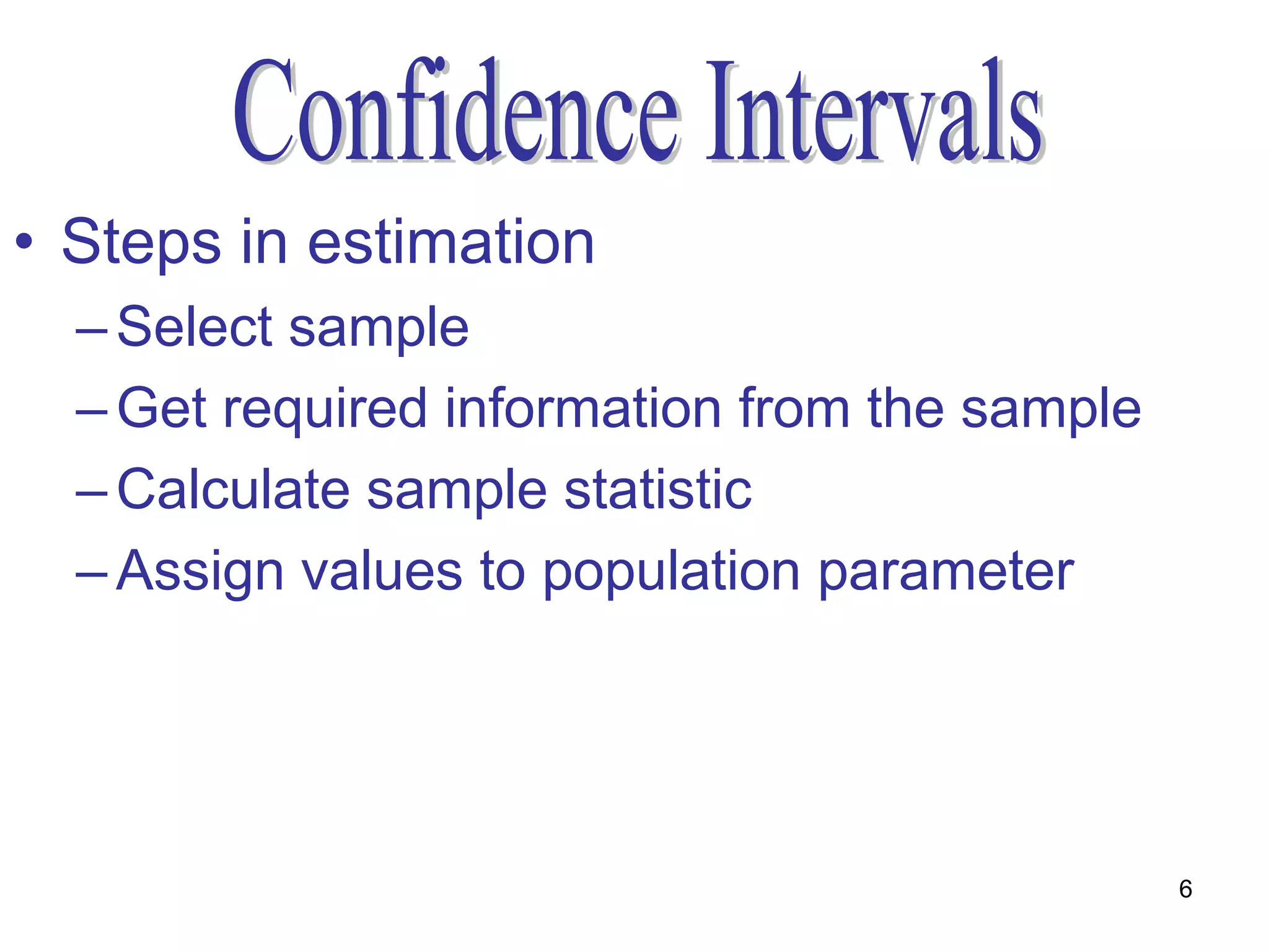
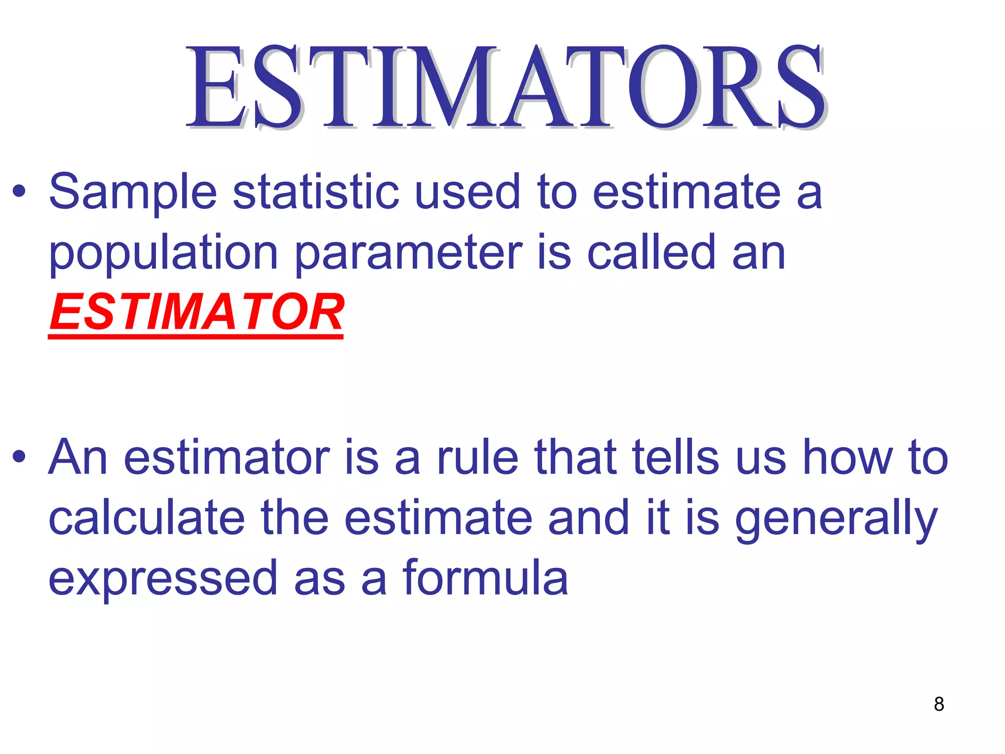
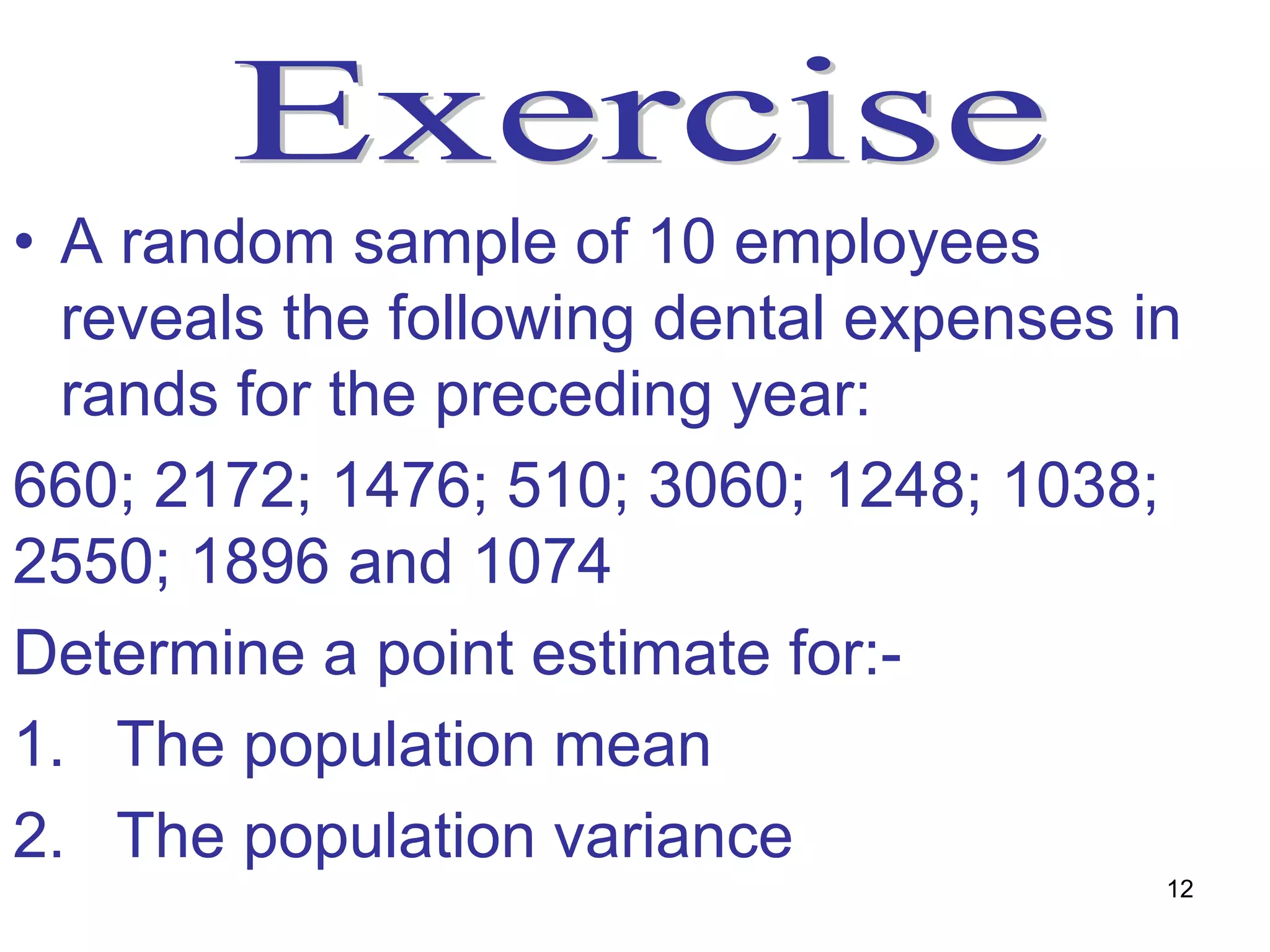
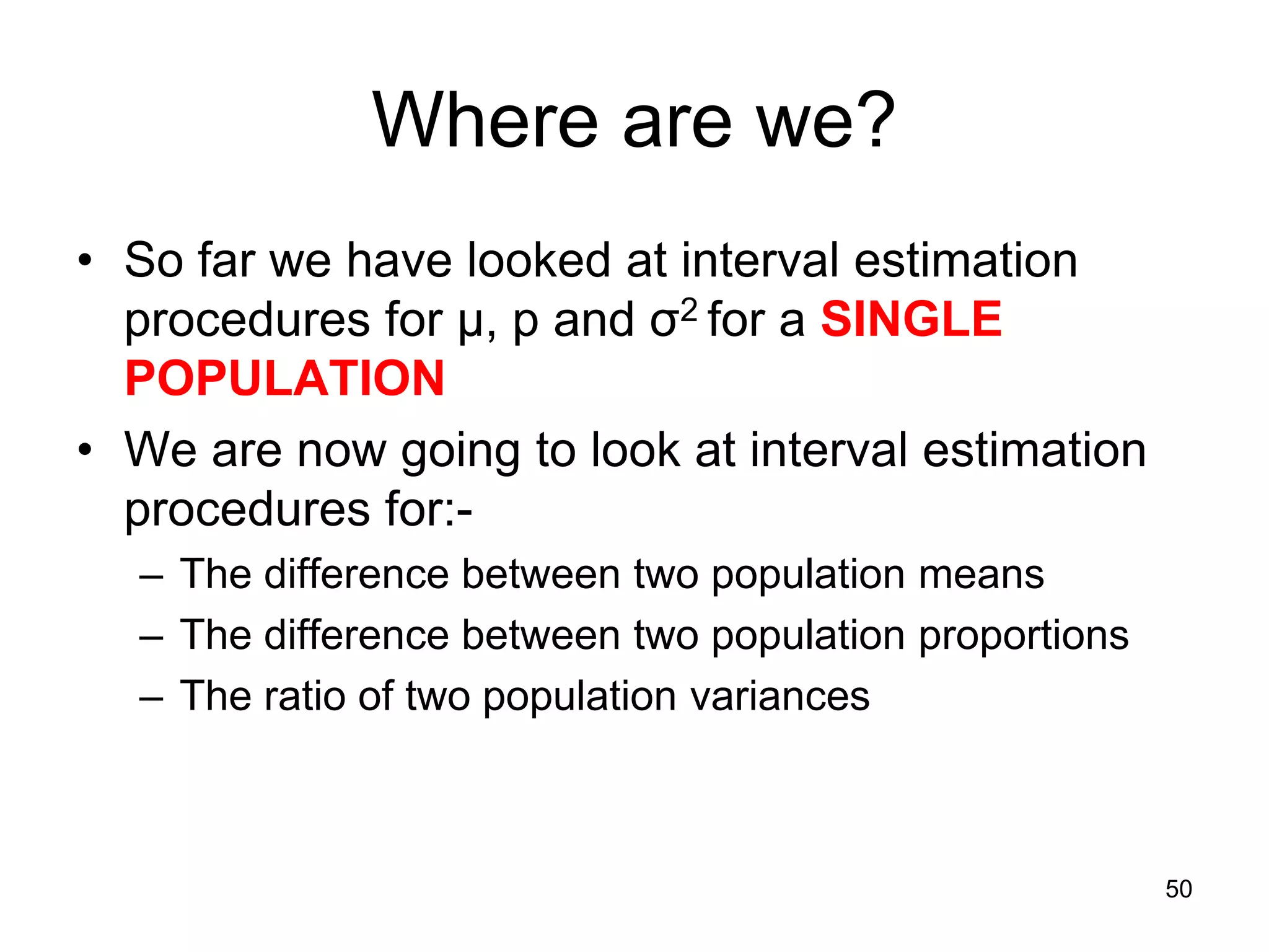
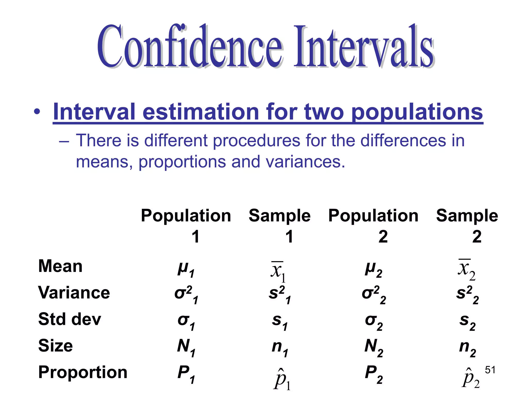
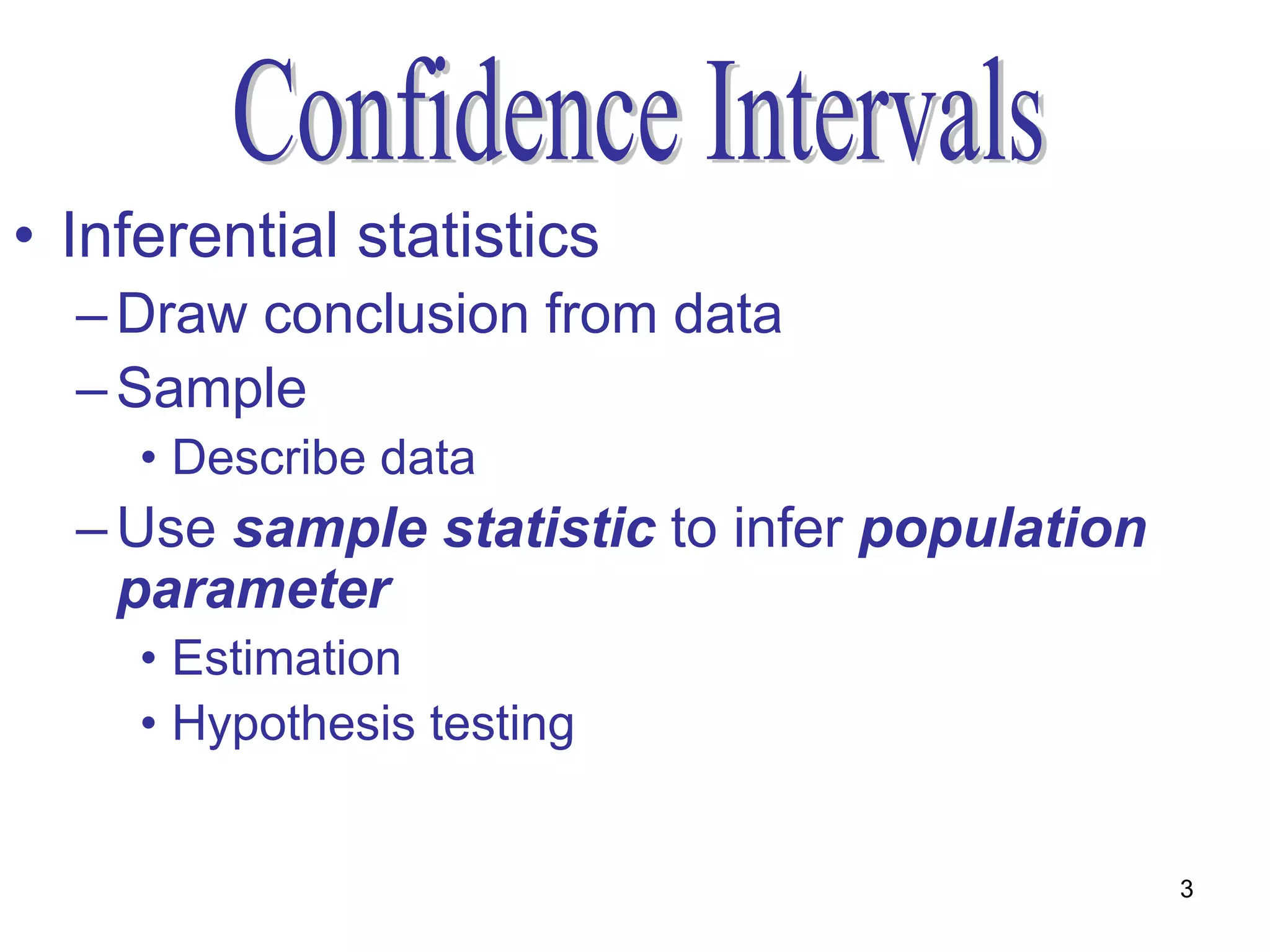
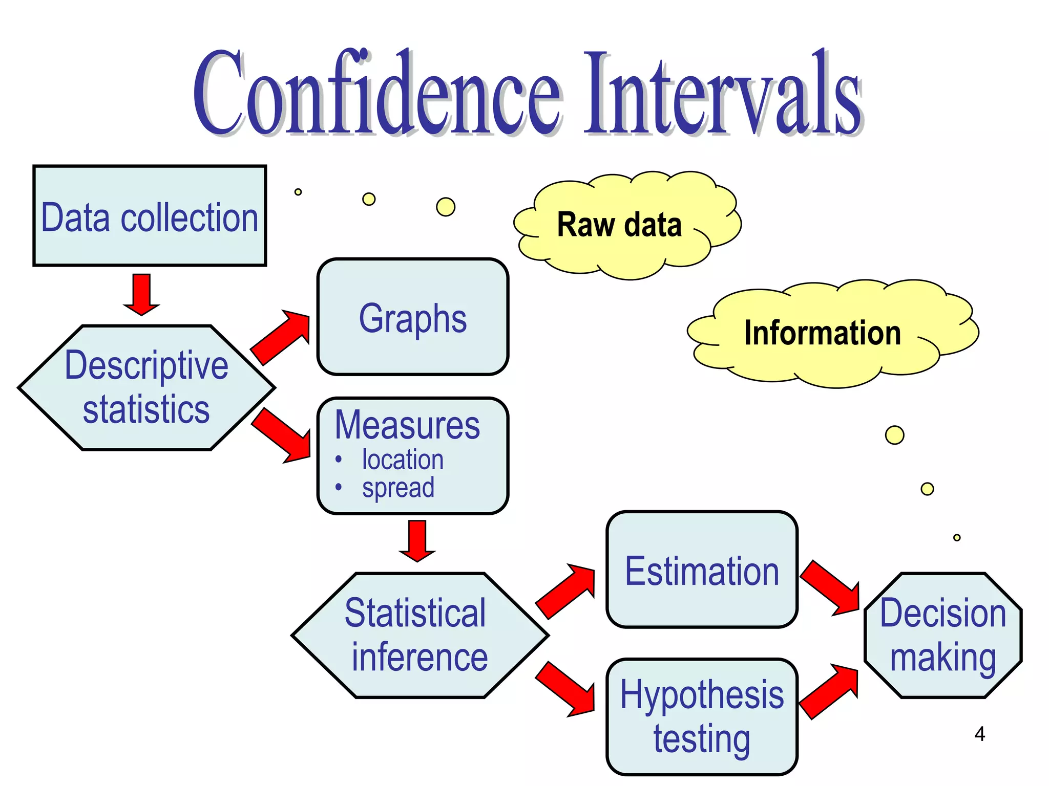
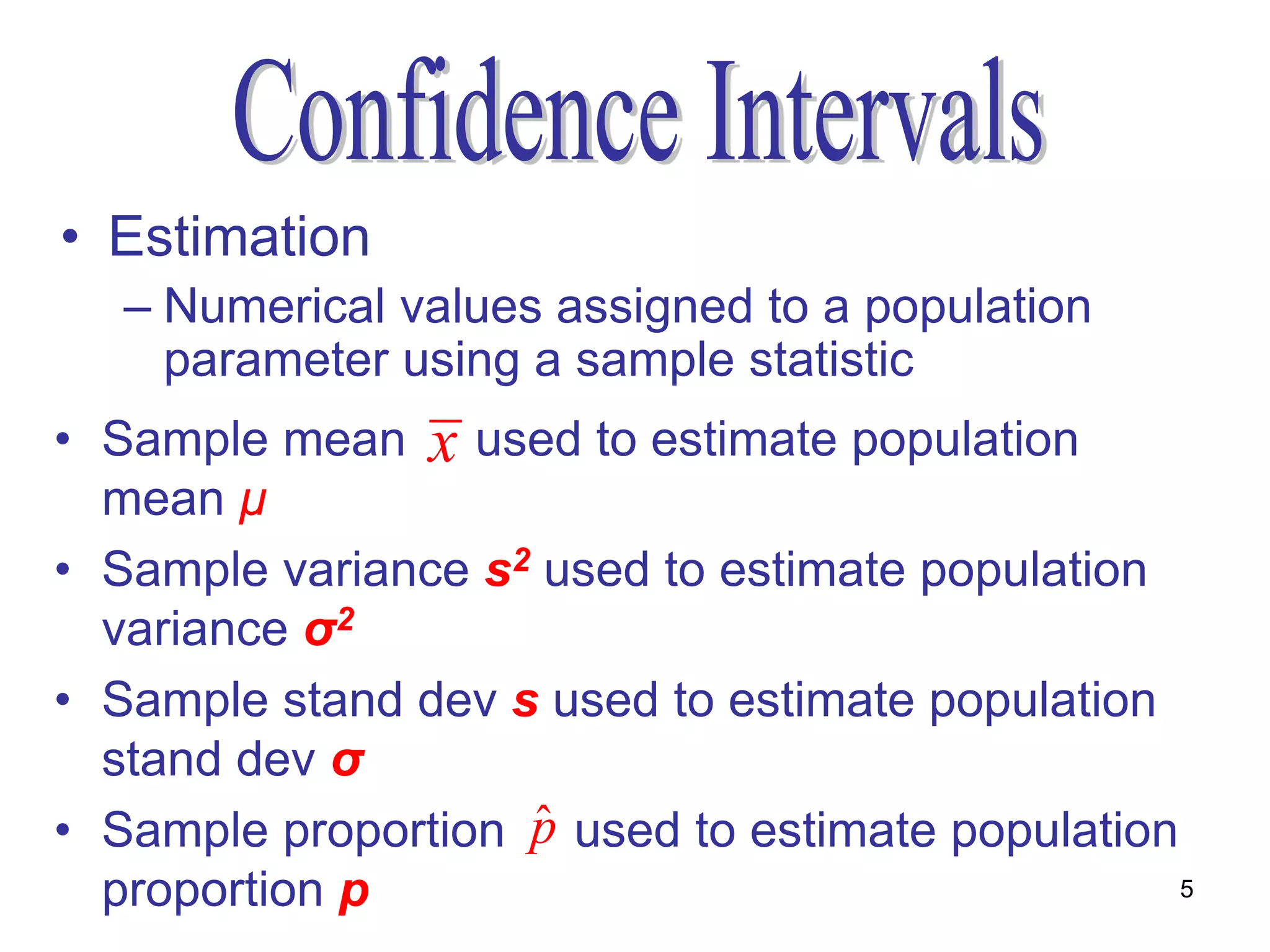
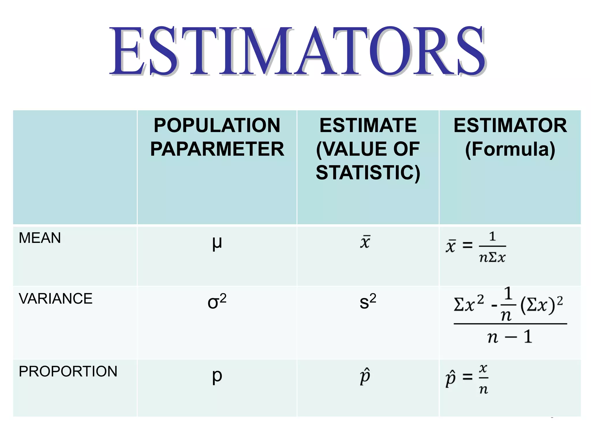
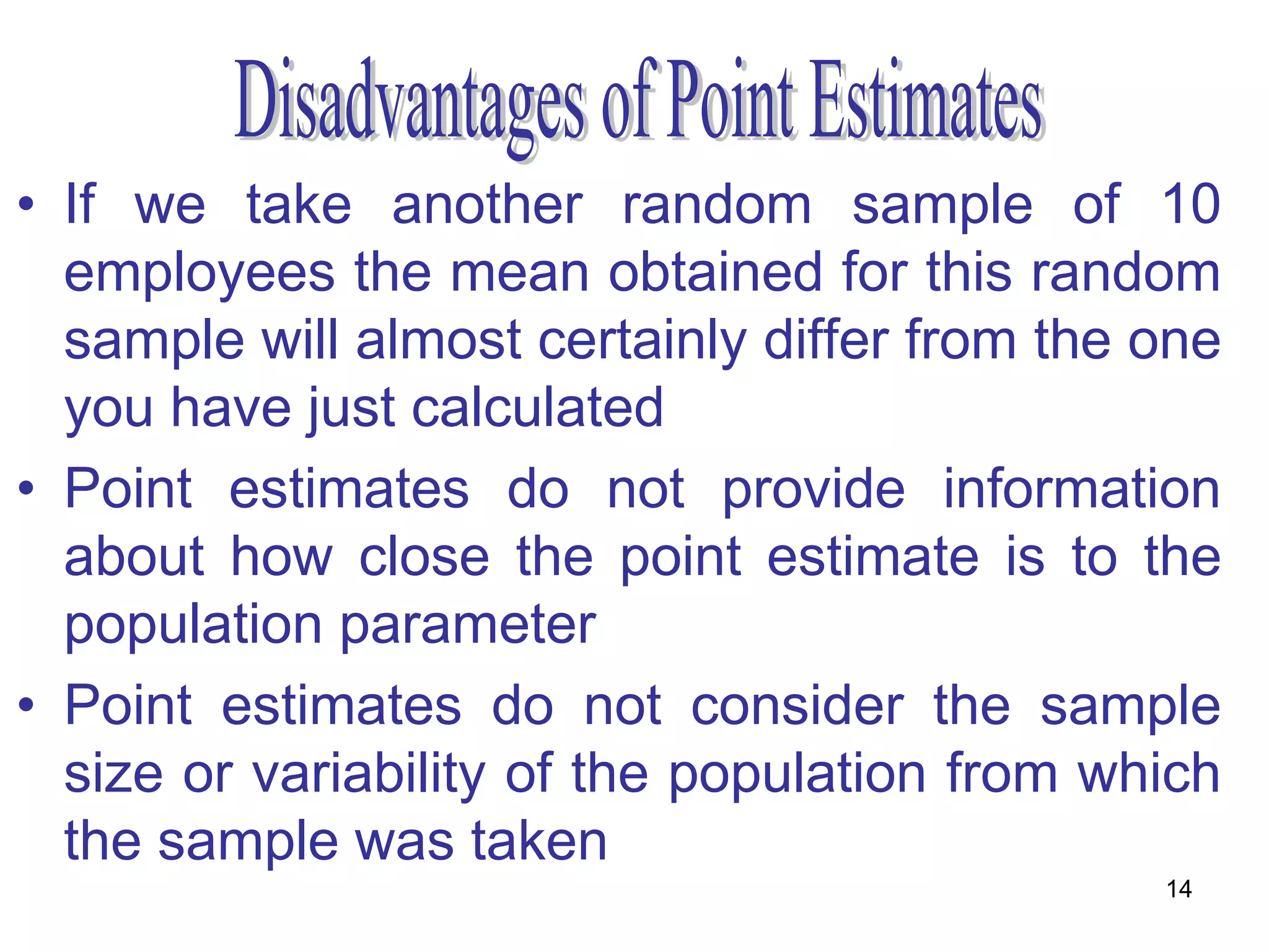
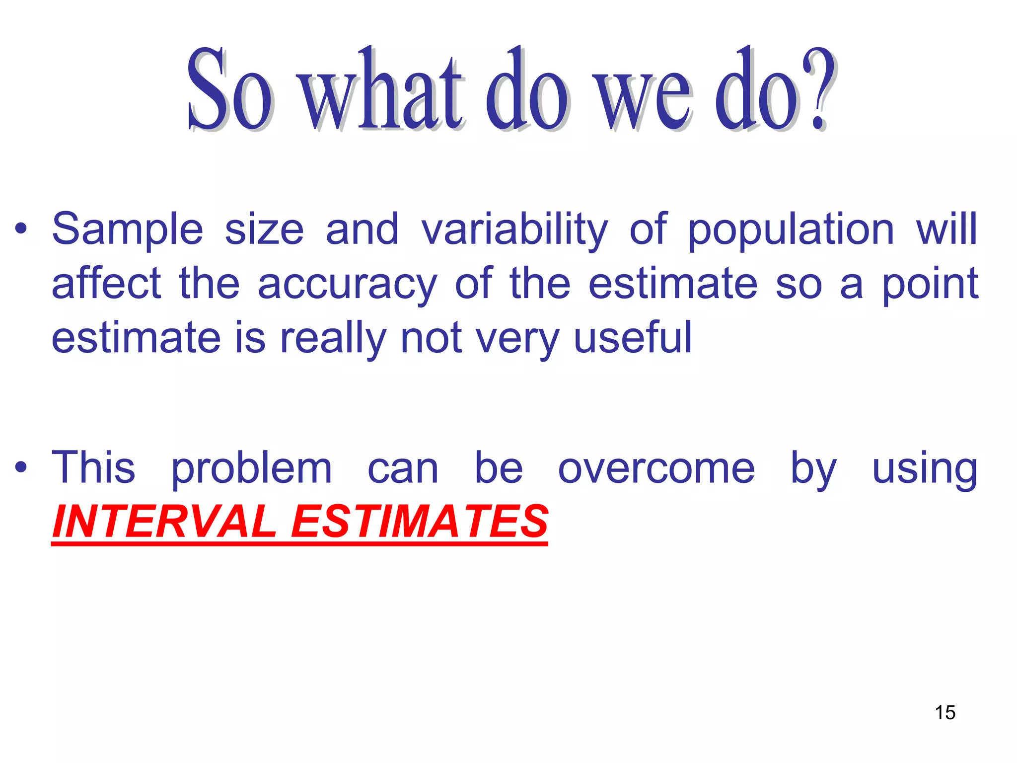
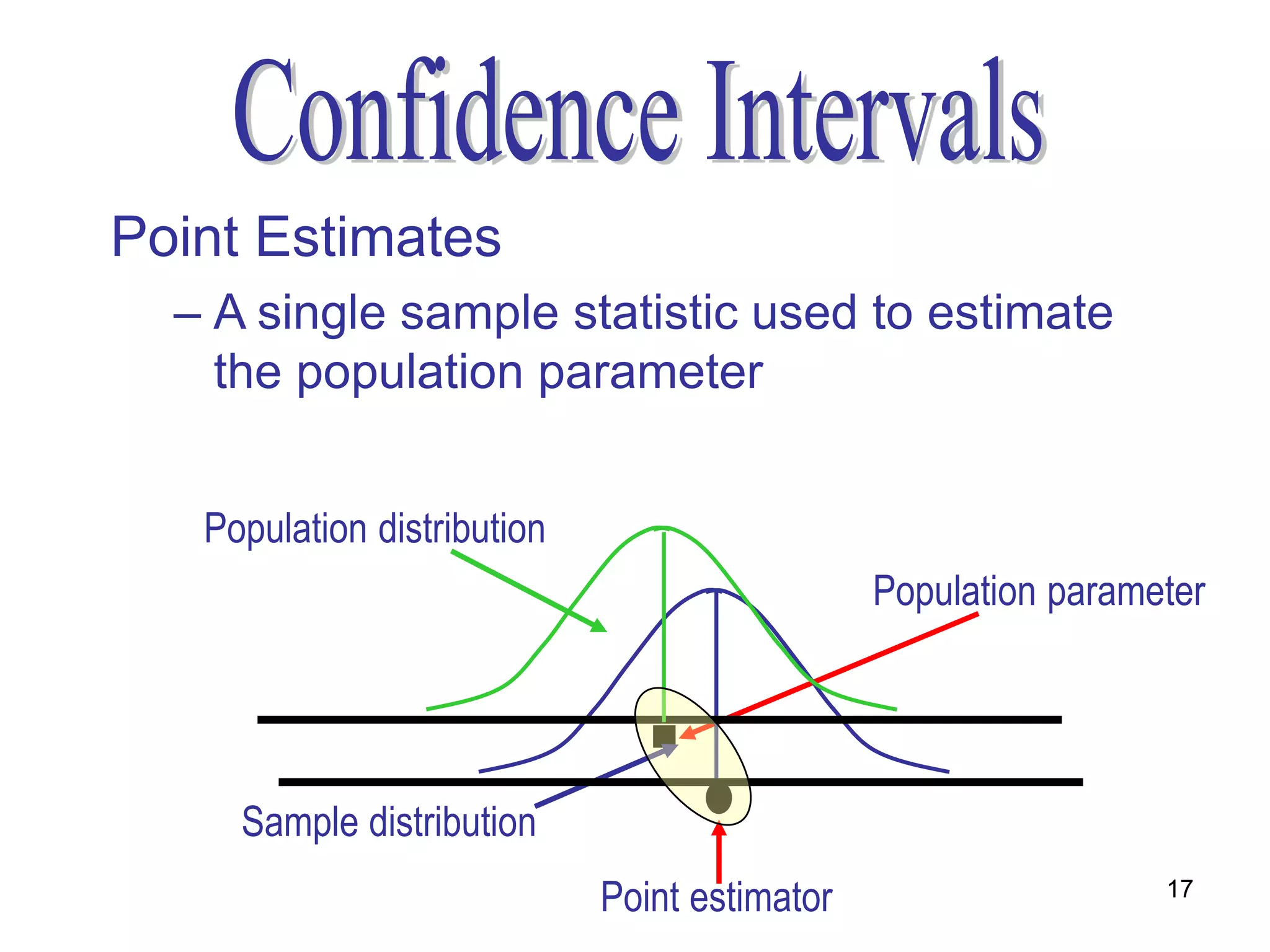
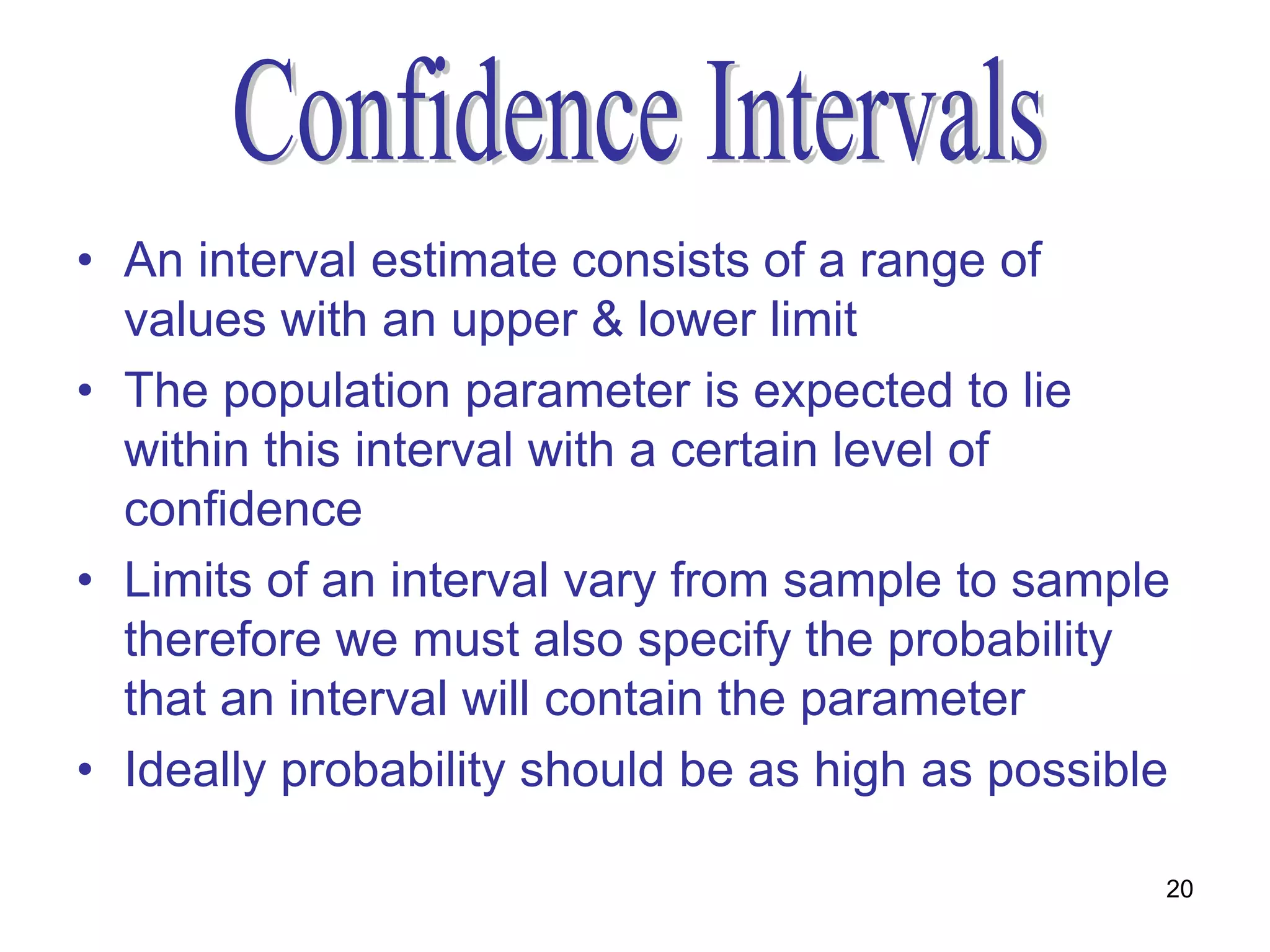
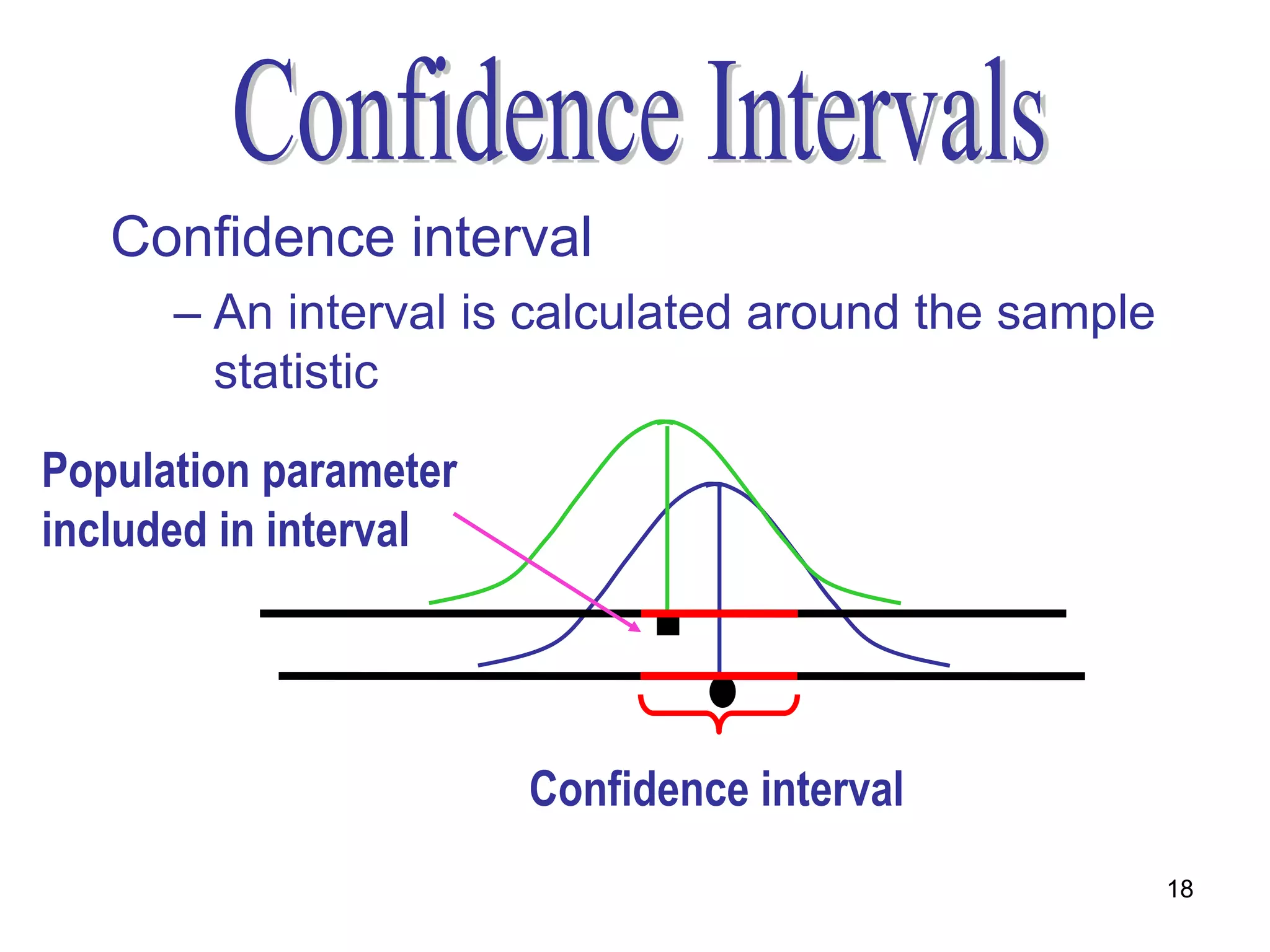
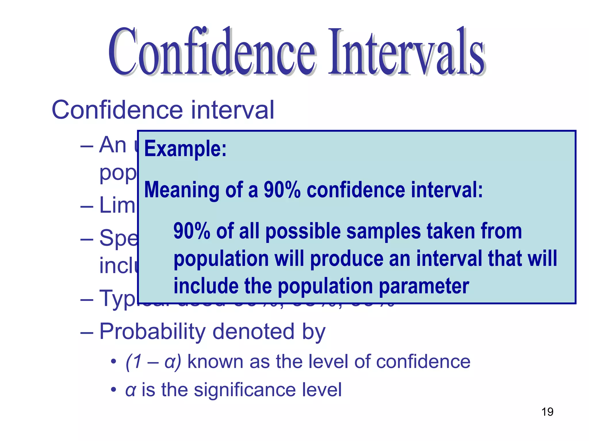
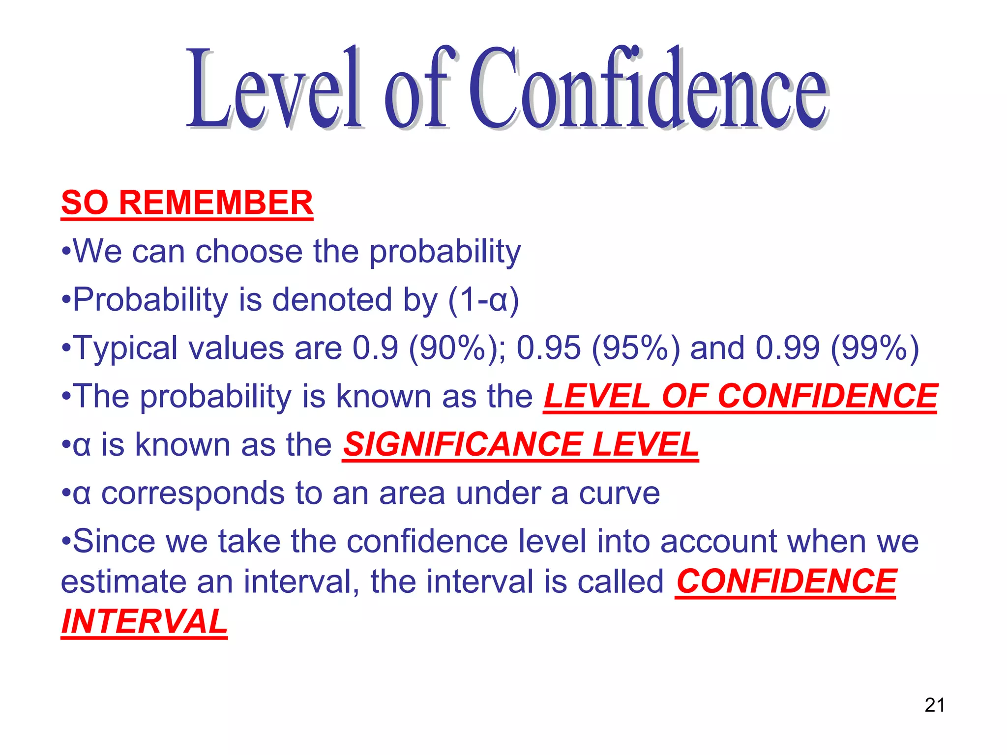
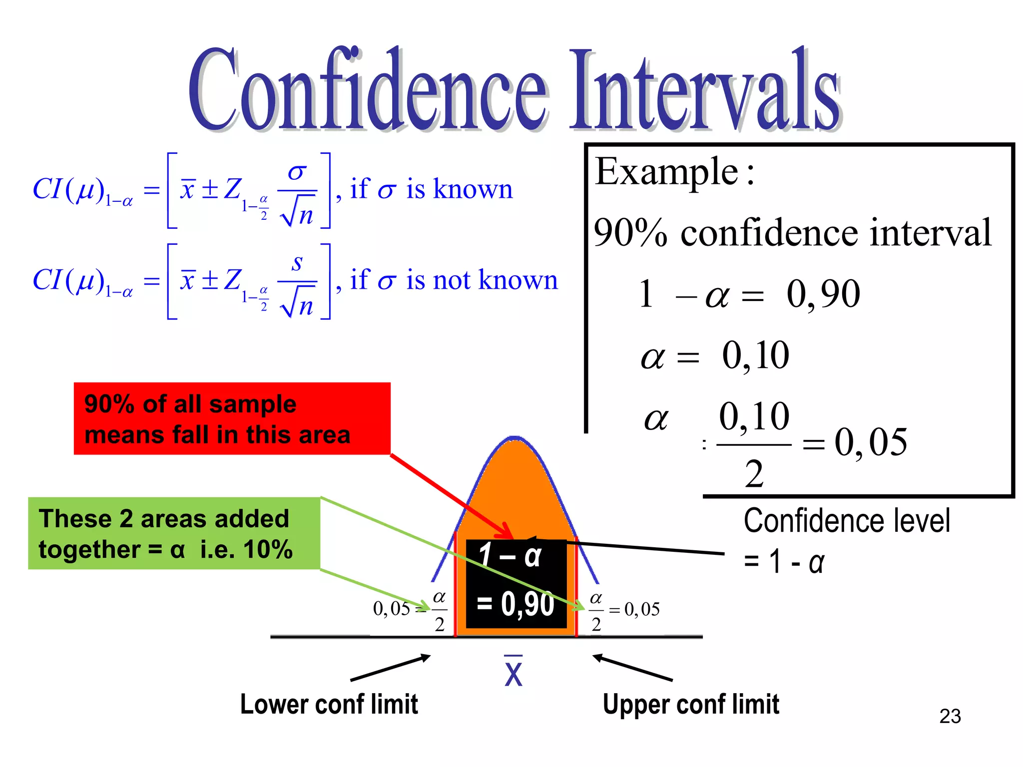
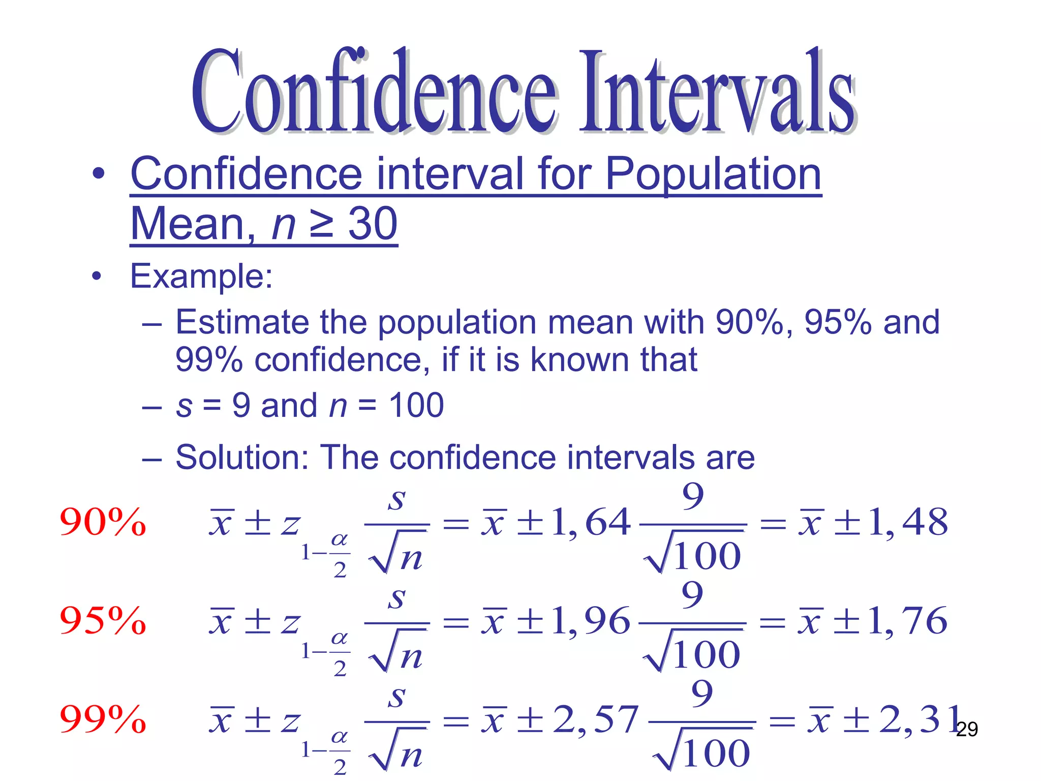
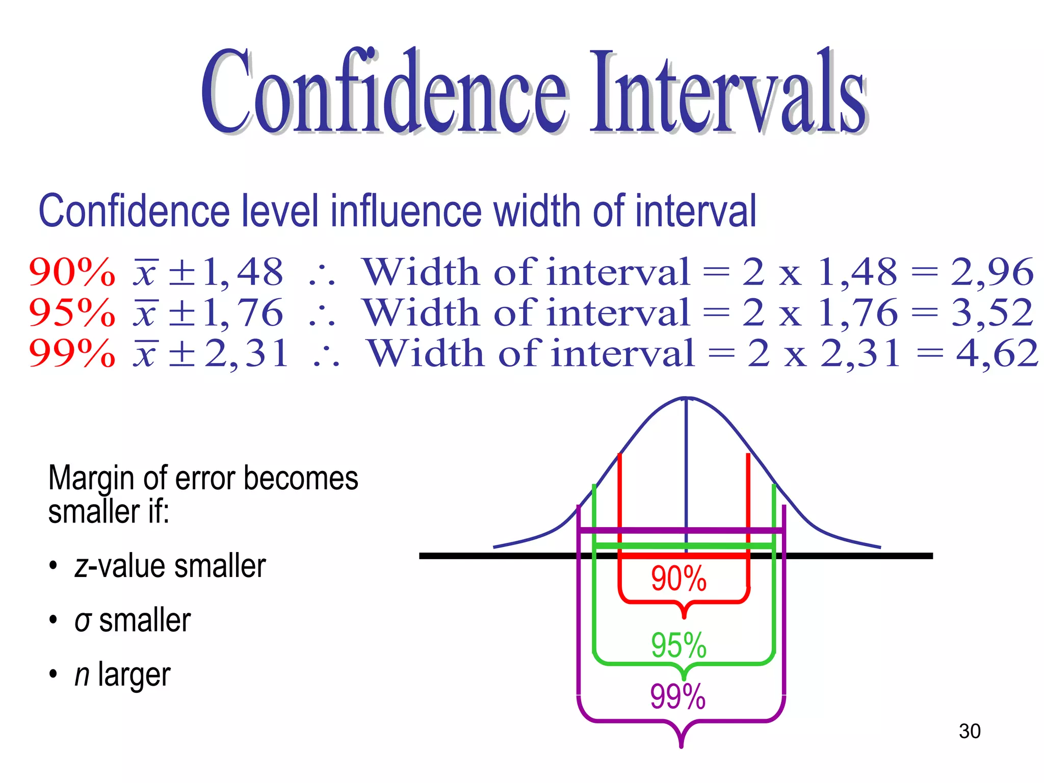
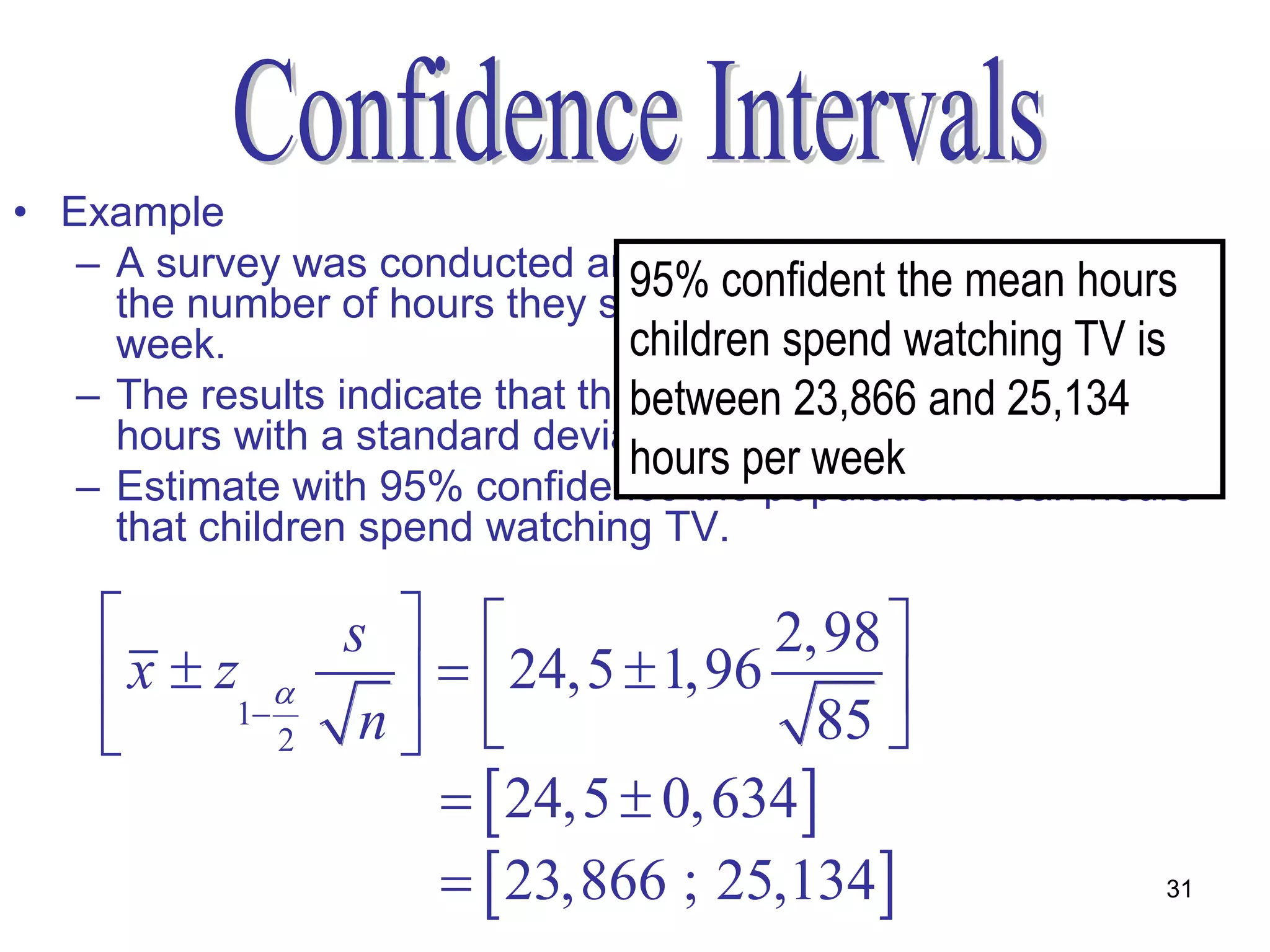
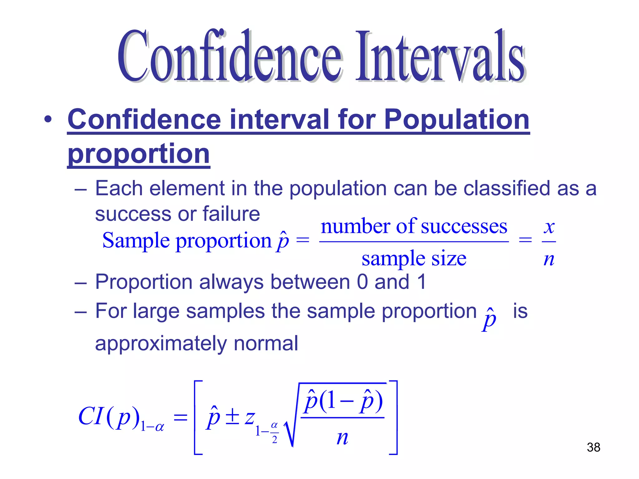
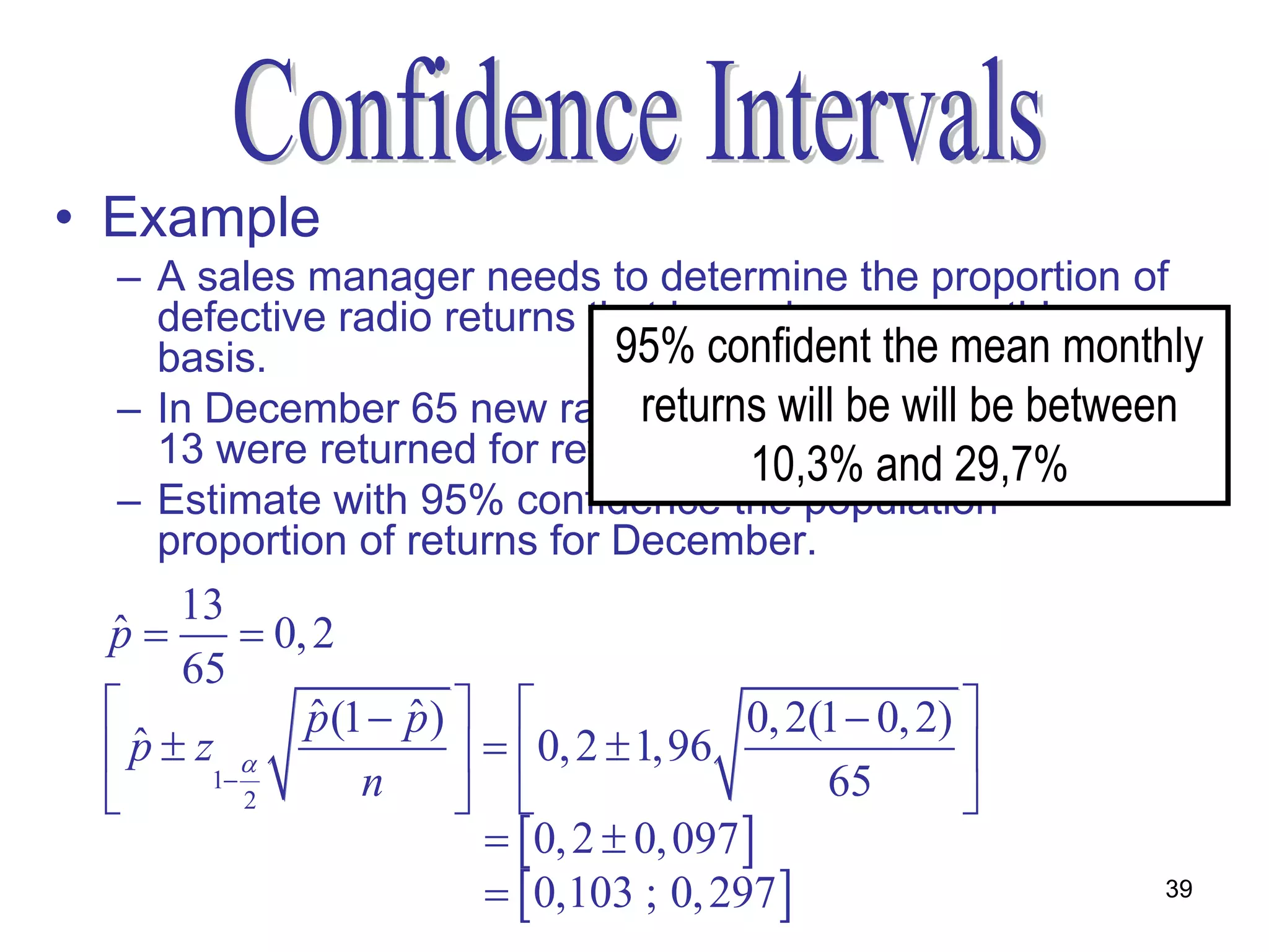
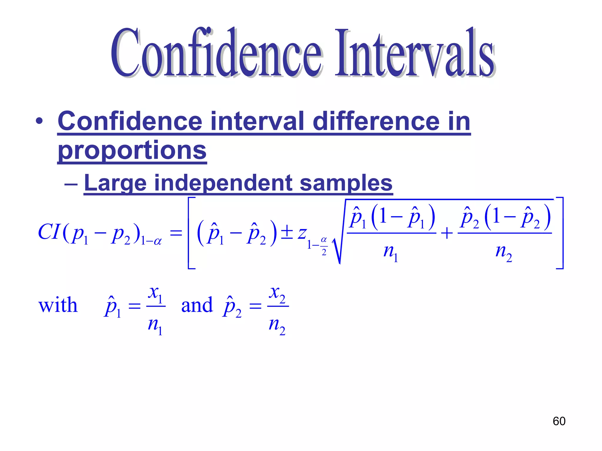
This document discusses statistical concepts such as parameters, statistics, descriptive statistics, estimation, and hypothesis testing. It provides examples of: - Point estimates and interval estimates used to estimate population parameters from sample statistics. Point estimates provide a single value while interval estimates provide a range of values. - Confidence intervals which specify a range of values that is expected to contain the population parameter a certain percentage of times, known as the confidence level. Common confidence levels are 90%, 95%, and 99%. 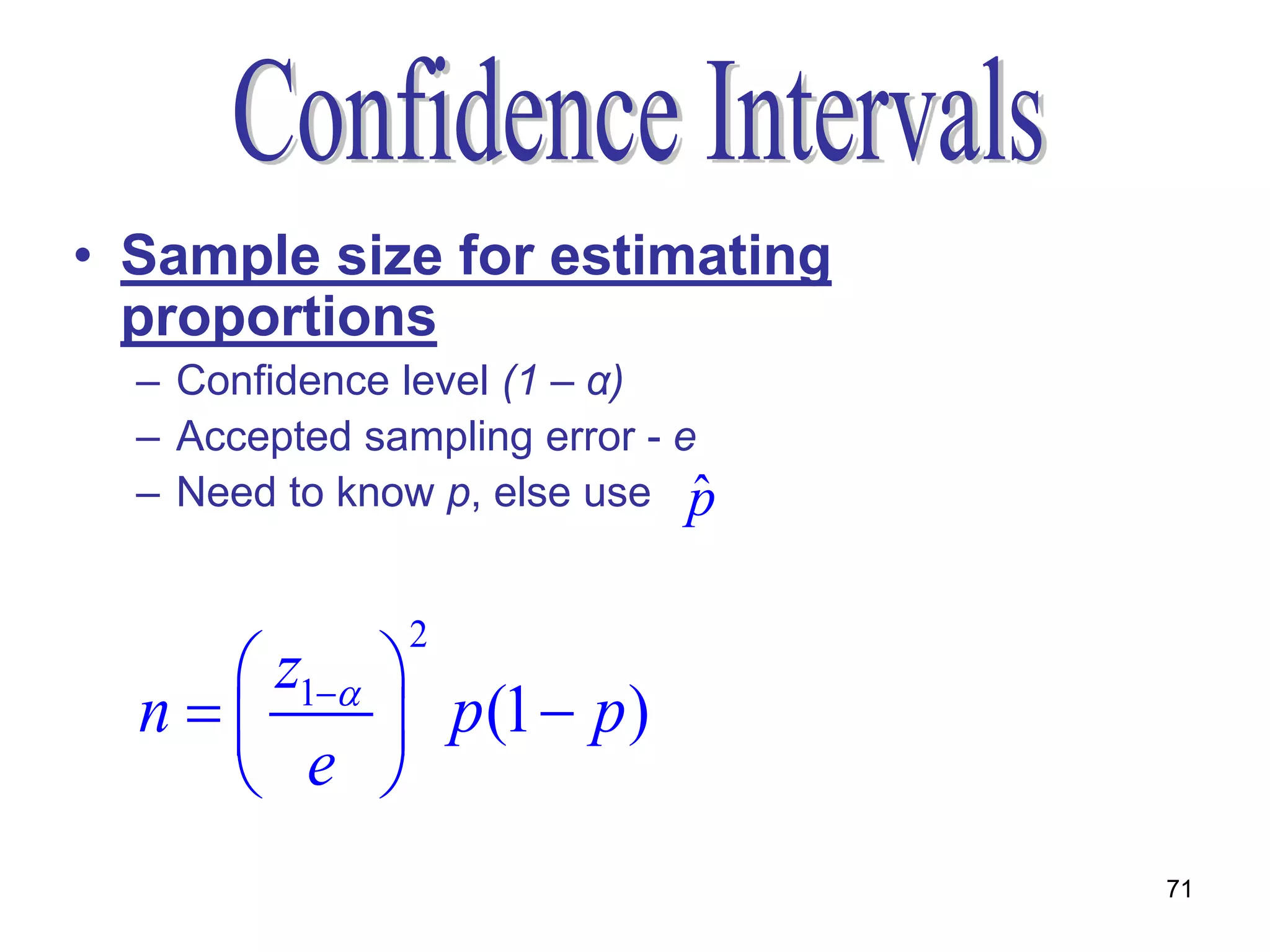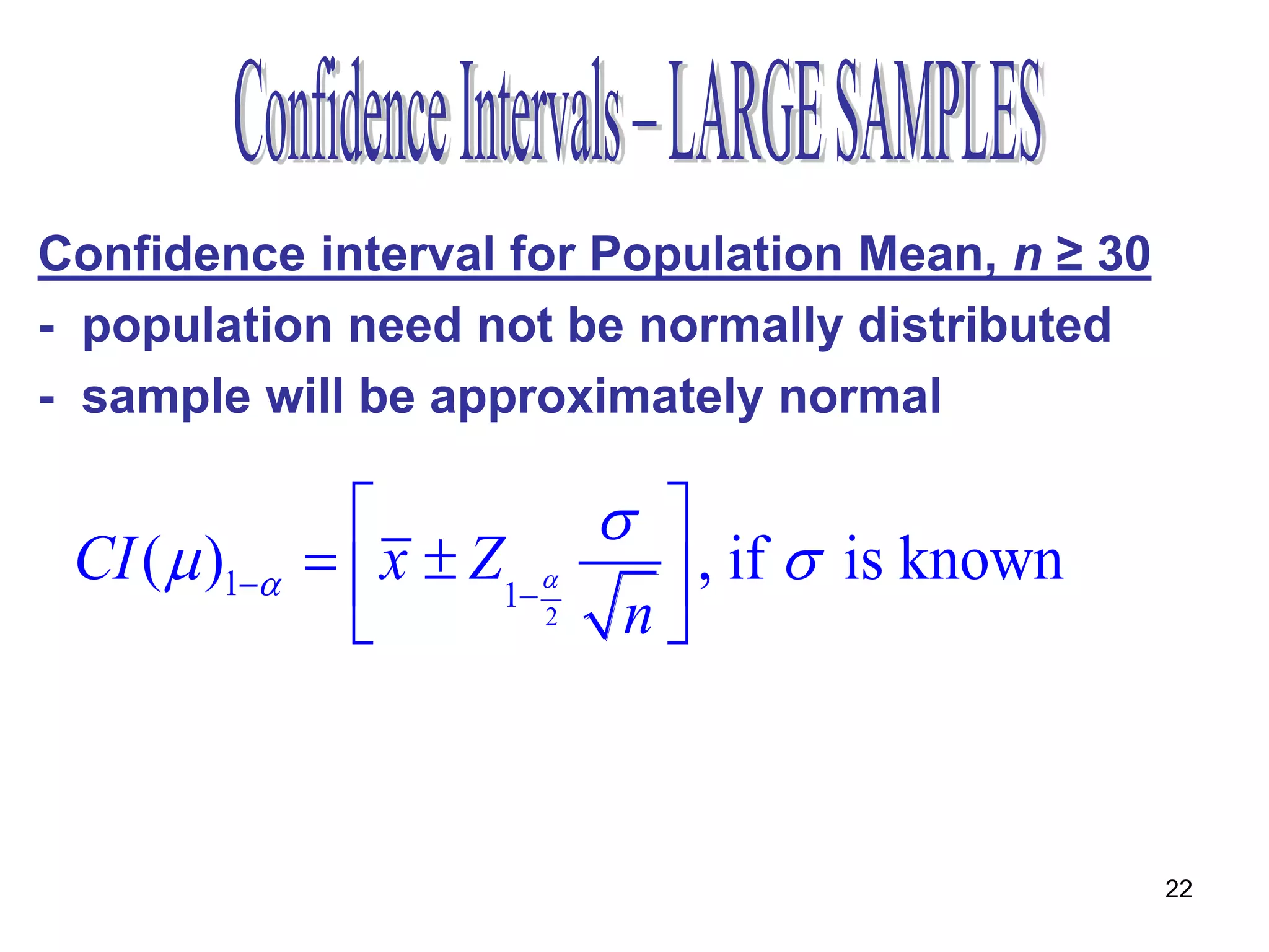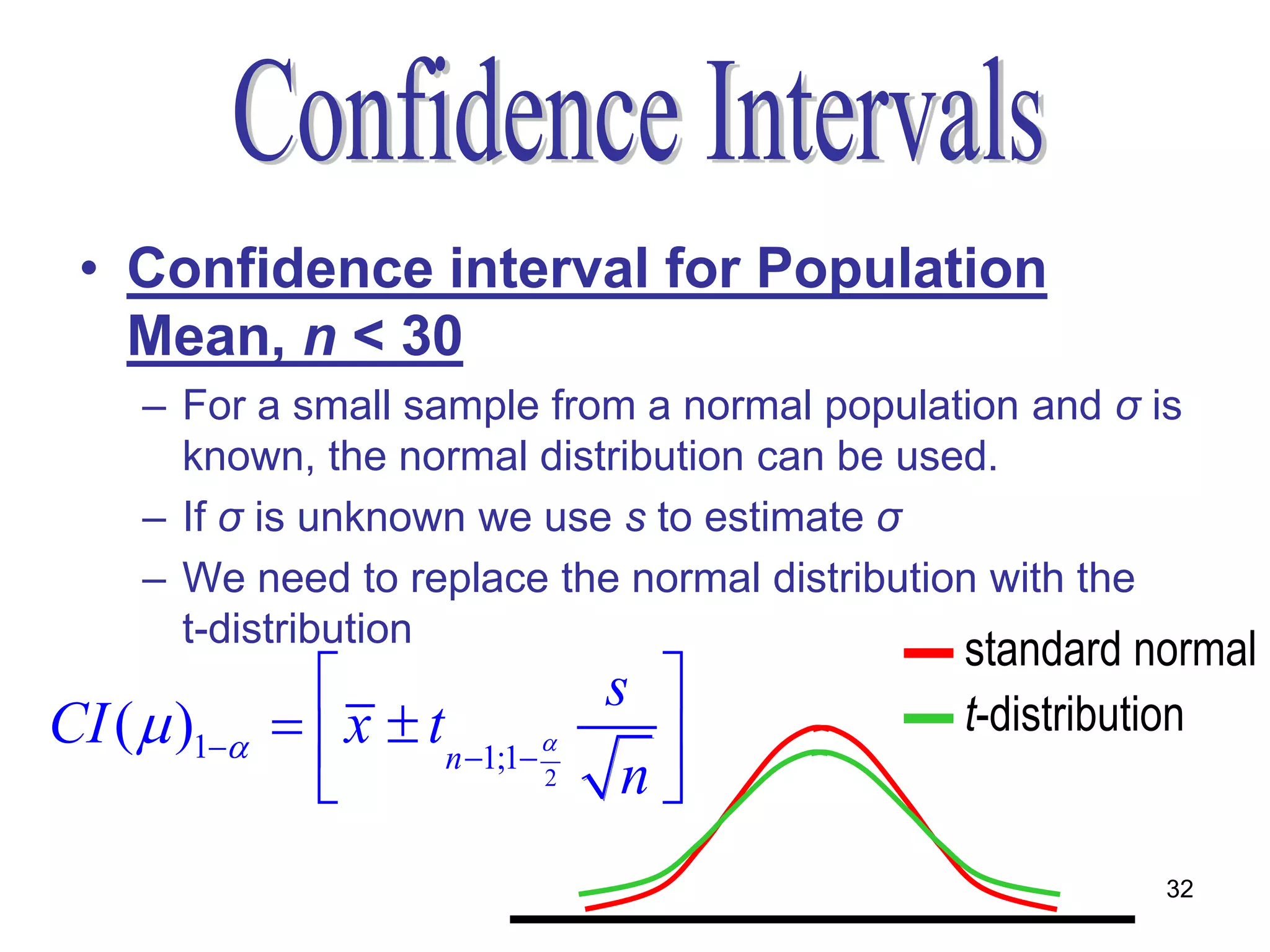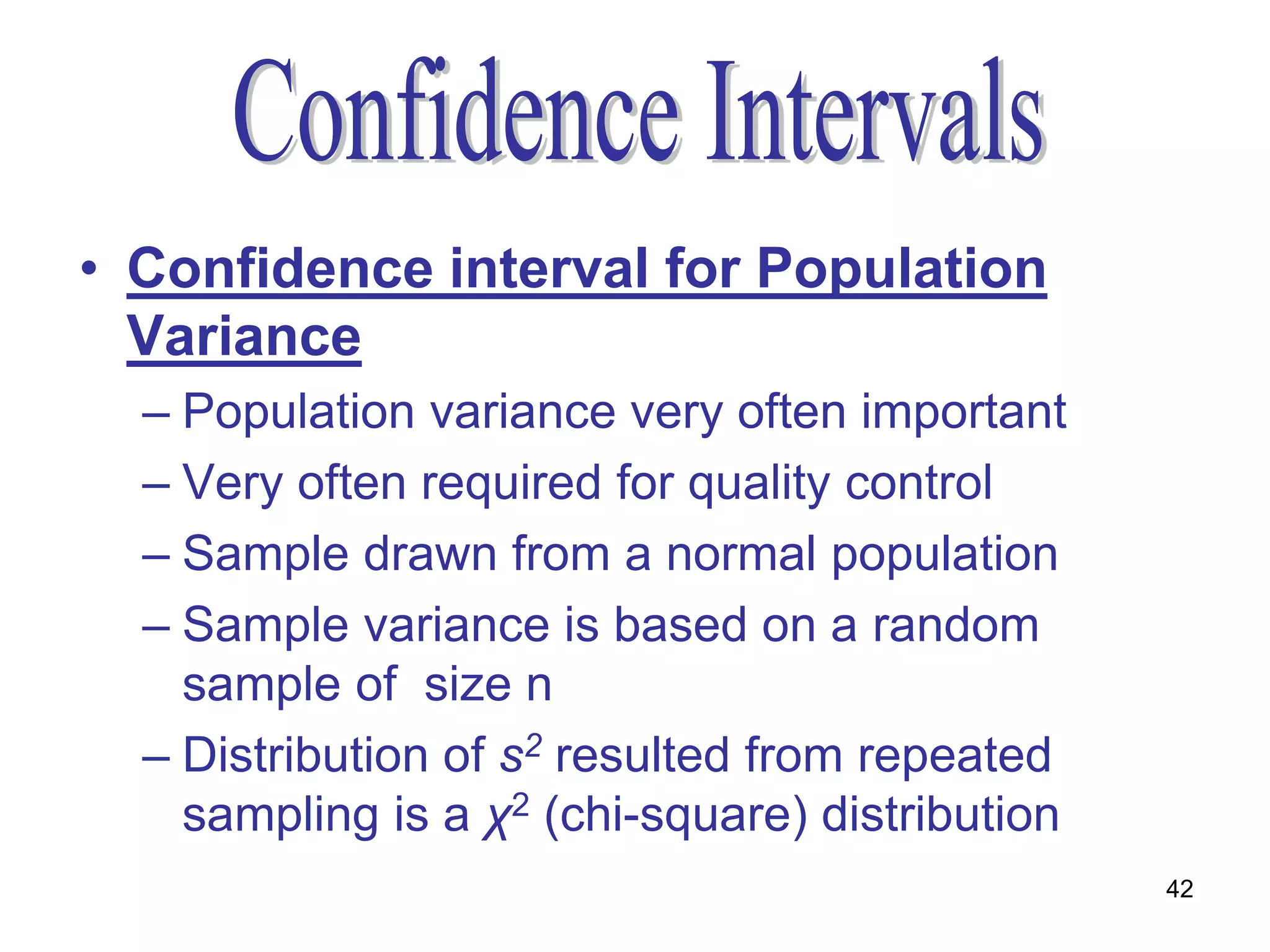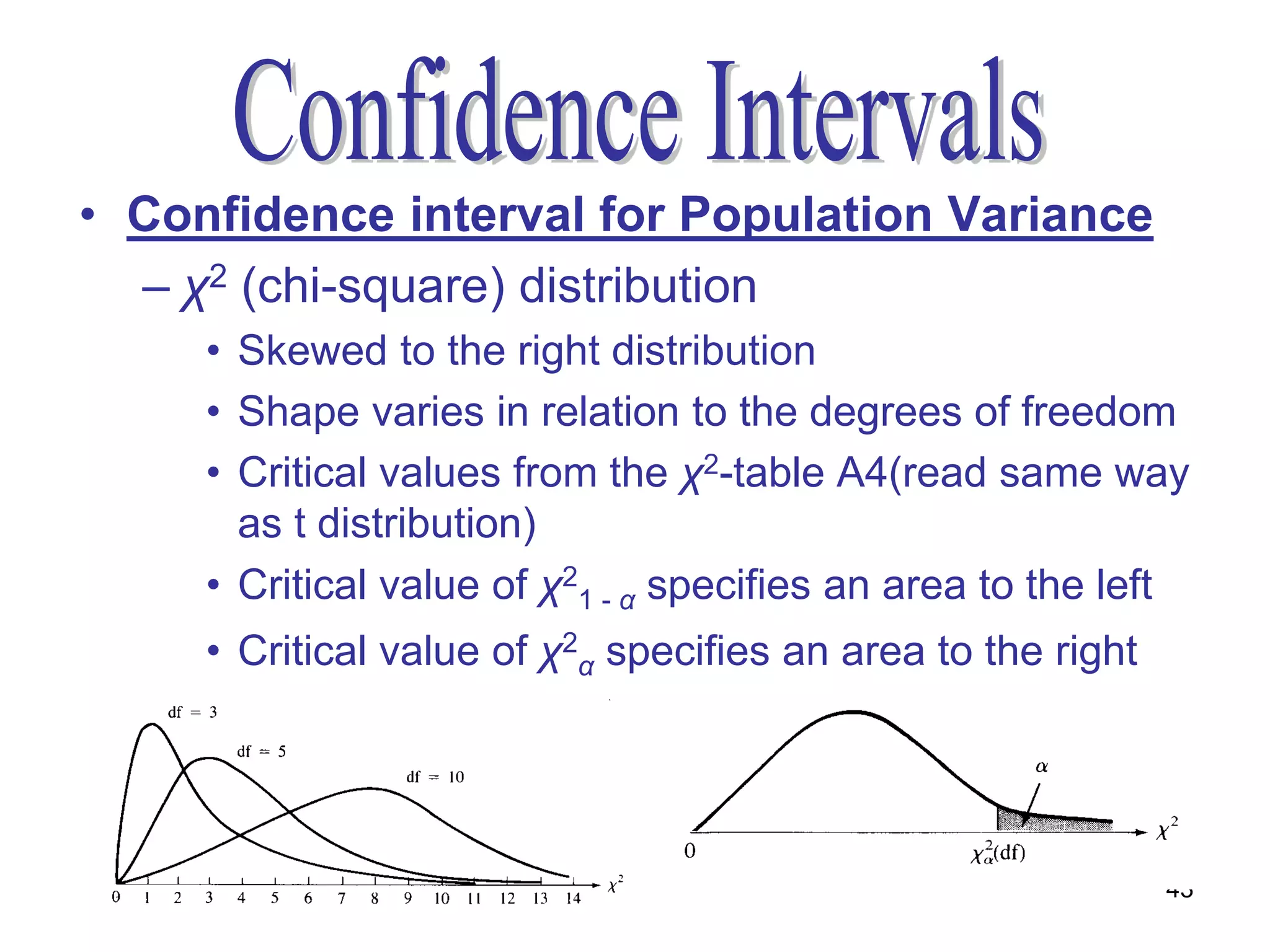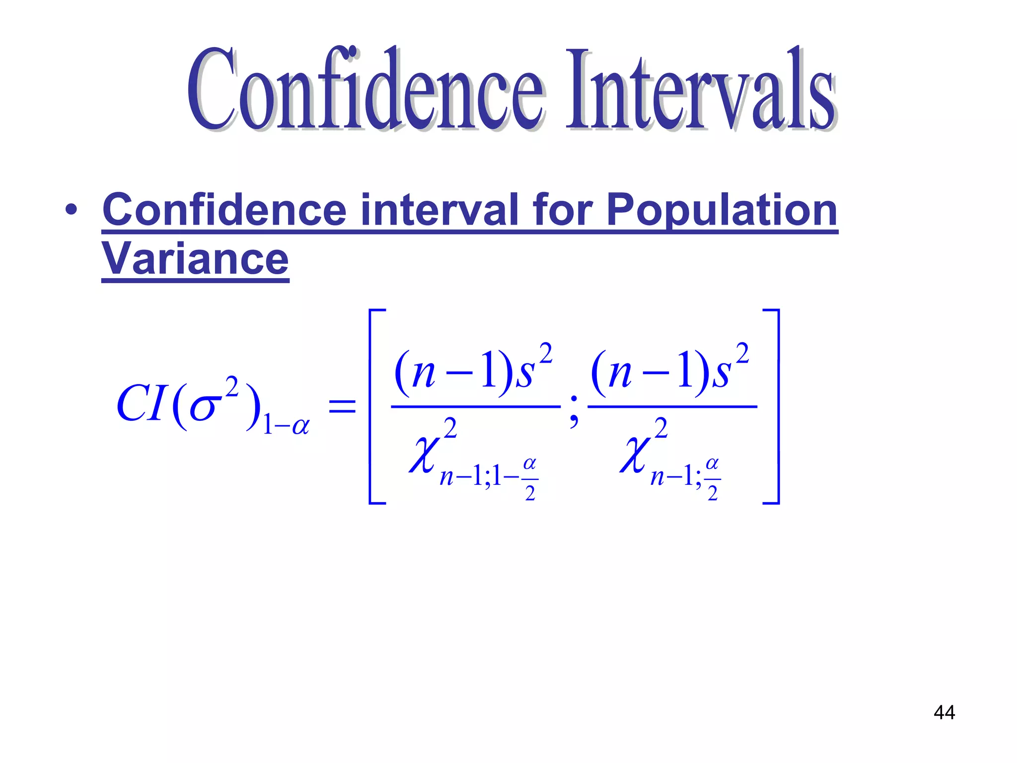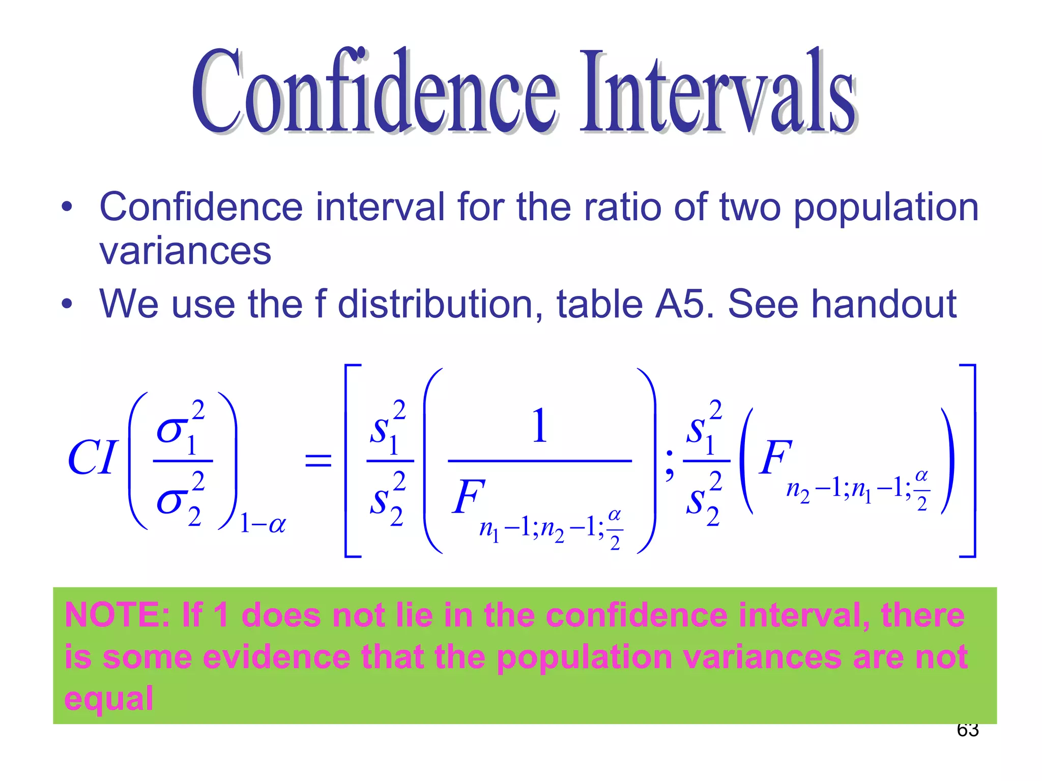- Formulas for constructing confidence intervals for the population mean, proportion, and variance based on the sample statistic, sample size, confidence level, and whether the population standard deviation is known.

1. 1

2. • A PARAMETER is a number that
describes a population statistic
• A STATISTIC is a number that describes
a characteristic in the sample data
2

3. • Inferential statistics
– Draw conclusion from data
– Sample
• Describe data
– Use sample statistic to infer population
parameter
• Estimation
• Hypothesis testing
3

4. Data collection Raw data
Graphs Information
Descriptive
statistics Measures
• location
• spread
Estimation
Statistical Decision
inference making
Hypothesis
testing 4

5. • Estimation
– Numerical values assigned to a population
parameter using a sample statistic
• Sample mean x used to estimate population
mean μ
• Sample variance s2 used to estimate population
variance σ2
• Sample stand dev s used to estimate population
stand dev σ
ˆ
• Sample proportion p used to estimate population
proportion p 5

6. • Steps in estimation
– Select sample
– Get required information from the sample
– Calculate sample statistic
– Assign values to population parameter
6

7. • Read example 7.1 page 214
7

8. • Sample statistic used to estimate a
population parameter is called an
ESTIMATOR
• An estimator is a rule that tells us how to
calculate the estimate and it is generally
expressed as a formula
8

9. POPULATION ESTIMATE ESTIMATOR
PAPARMETER (VALUE OF (Formula)
STATISTIC)
MEAN µ
VARIANCE σ2 s2
PROPORTION p
9

10. • Two types of estimate:-
–Point estimates
–Interval estimates
10

11. • A single number that is calculated from
sample data
• Resulting number then used to estimate
the true value of the corresponding
population parameter
11

12. • A random sample of 10 employees
reveals the following dental expenses in
rands for the preceding year:
660; 2172; 1476; 510; 3060; 1248; 1038;
2550; 1896 and 1074
Determine a point estimate for:-
1. The population mean
2. The population variance
12

13. • Answer p215
13

14. • If we take another random sample of 10
employees the mean obtained for this random
sample will almost certainly differ from the one
you have just calculated
• Point estimates do not provide information
about how close the point estimate is to the
population parameter
• Point estimates do not consider the sample
size or variability of the population from which
the sample was taken
14

15. • Sample size and variability of population will
affect the accuracy of the estimate so a point
estimate is really not very useful
• This problem can be overcome by using
INTERVAL ESTIMATES
15

16. • No 1 – 6 page 216
16

17. Point Estimates
– A single sample statistic used to estimate
the population parameter
Population distribution
Population parameter
Sample distribution
Point estimator 17

18. Confidence interval
– An interval is calculated around the sample
statistic
Population parameter
included in interval
Confidence interval
18

19. Confidence interval
– An upper and lower limit within in which the
Example:
population parameter is expected to lie
Meaning of a 90% confidence interval:
– Limits will vary from sample to sample
– Specify90% of all possible samples taken from
the probability that the interval will
include population will produce an interval that will
the parameter
include the population parameter
– Typical used 90%, 95%, 99%
– Probability denoted by
• (1 – α) known as the level of confidence
• α is the significance level
19

20. • An interval estimate consists of a range of
values with an upper & lower limit
• The population parameter is expected to lie
within this interval with a certain level of
confidence
• Limits of an interval vary from sample to sample
therefore we must also specify the probability
that an interval will contain the parameter
• Ideally probability should be as high as possible
20

21. SO REMEMBER
•We can choose the probability
•Probability is denoted by (1-α)
•Typical values are 0.9 (90%); 0.95 (95%) and 0.99 (99%)
•The probability is known as the LEVEL OF CONFIDENCE
•α is known as the SIGNIFICANCE LEVEL
•α corresponds to an area under a curve
•Since we take the confidence level into account when we
estimate an interval, the interval is called CONFIDENCE
INTERVAL
21

22. Confidence interval for Population Mean, n ≥ 30
- population need not be normally distributed
- sample will be approximately normal
  
CI (  )1   x  Z1   , if  is known
 2 n
 s 
CI (  )1   x  Z1   , if  is not known
 2 n
22

23.    Example :
CI (  )1   x  Z1   , if  is known
 2 n
90% confidence interval
 s 
CI (  )1   x  Z1   , if  is not known
 2 n 1 –   0,90
  0,10
1
90% of all sample
 0,10
means fall in this area   0, 05
2 2
These 2 areas added Confidence level
together = α i.e. 10% 1–α =1-α

1-α   0, 05

0, 05 
2
= 0,90 2
2
x
Lower conf limit Upper conf limit 23

24. 24

25. See handout
25

26. A random sample of repair costs for 150
hotel rooms gave a mean repair cost of
R84.30 and a standard deviation of R37.20.
Construct a 95% confidence interval for the
mean repair cost for a population of 2000
hotel rooms
26

27. Example 7.3 p218
27

28. • Four commonly used confidence levels

1-α α 2 z
0,9 0,1 0,05 1,64
0,95 0,05 0,025 1,96
0,98 0,02 0,01 2,33
0,99 0,01 0,005 2,57
28

29. • Confidence interval for Population
Mean, n ≥ 30
• Example:
– Estimate the population mean with 90%, 95% and
99% confidence, if it is known that
– s = 9 and n = 100
– Solution: The confidence intervals are
s 9
90% xz   x  1, 64  x  1, 48
1 n 100
2
s 9
95% xz   x  1, 96  x  1, 76
1 n 100
2
s 9
99% xz   x  2, 57  x  2, 31 29
1 n 100
2

30. Confidence level influence width of interval
90% x  1, 48  Width of interval = 2 x 1,48 = 2,96
95% x  1, 76  Width of interval = 2 x 1,76 = 3,52
99% x  2, 31  Width of interval = 2 x 2,31 = 4,62
Margin of error becomes
smaller if:
• z-value smaller 90%
• σ smaller
95%
• n larger
99%
30

31. • Example
– A survey was conducted amongst 85 childrenmean hours
95% confident the to determine
the number of hours they spend in front of the TV every
week. children spend watching TV is
– The results indicate that thebetween 23,866 and 25,134 24,5
mean for the sample was
hours with a standard deviation of 2,98 hours.
hours per week
– Estimate with 95% confidence the population mean hours
that children spend watching TV.
 s   2,98 
 x  z1     24,5  1,96 
 2 n  85 
  24,5  0, 634
  23,866 ; 25,134 31

32. • Confidence interval for Population
Mean, n < 30
– For a small sample from a normal population and σ is
known, the normal distribution can be used.
– If σ is unknown we use s to estimate σ
– We need to replace the normal distribution with the
t-distribution
▬ standard normal
 s 
CI (  )1   x  tn 1;1  
▬ t-distribution
 2 n
32

33. t Distribution
• Refer to handout on how to read the
critical value t n-1; 1- 𝛼
2
33

34. • Example
– The manager of a small departmental store is concerned
about the decline of his weekly sales.
99% confident the mean weekly
– He calculated the average and standard deviation of his
sales for the past 12 weeks, x =sales will be between
R12400 and s = R1346
– Estimate with 99% confidence the populationR13 606,86
R11 193,14 and mean sales
of the departmental store.
t11;0.995
 s   1346 
 x  tn 1;1    12400  3,106 
 2 n  12 
 12400  1206,86
 11193,14 ; 13606,86  34

35. EXAMPLE 2
• A study of absenteeism among workers at
a local mine during the previous year was
carried out. A random sample of 25 miners
revealed a mean absenteeism of 9.7days
with a variance of 16 days. Construct a
confidence interval for the average
number of days of absence for miners for
last year. Assume the population is
normally distributed.
35

36. EXAMPLE 2 - ANSWER
• Example 7.6, page 222 textbook
36

37. CLASSWORK
• Do concept questions 7 – 19, page 223
textbook
37

38. • Confidence interval for Population
proportion
– Each element in the population can be classified as a
success or failure
number of successes x
ˆ
Sample proportion p = =
sample size n
– Proportion always between 0 and 1
– For large samples the sample proportion ˆ
p is
approximately normal
 p (1  p ) 
ˆ ˆ
CI ( p )1   p  z1 
ˆ 
 2 n  38

39. • Example
– A sales manager needs to determine the proportion of
defective radio returns that is made on a monthly
basis. 95% confident the mean monthly
– In December 65 new radios werewill be will in January
returns sold and be between
13 were returned for rework. 10,3% and 29,7%
– Estimate with 95% confidence the population
proportion of returns for December.
13
p
ˆ  0, 2
65
 p (1  p )  
ˆ ˆ 0, 2(1  0, 2) 
 p  z1 
ˆ    0, 2  1,96 
 2 n   65 
  0, 2  0, 097 
  0,103 ; 0, 297  39

40. EXAMPLE 2
• A cellphone retailer is experiencing
problems with a high % of returns. The
quality control manager wants to estimate
the % of all sales that result in returns. A
sample of 40 sales showed that 8
cellphones were returned. Construct a
99% confidence interval for the % of all
sales that result in returns
40

41. EXAMPLE 2
• Answer – example 7.9 page 225, textbook
41

42. • Confidence interval for Population
Variance
– Population variance very often important
– Very often required for quality control
– Sample drawn from a normal population
– Sample variance is based on a random
sample of size n
– Distribution of s2 resulted from repeated
sampling is a χ2 (chi-square) distribution
42

43. • Confidence interval for Population Variance
– χ2 (chi-square) distribution
• Skewed to the right distribution
• Shape varies in relation to the degrees of freedom
• Critical values from the χ2-table A4(read same way
as t distribution)
• Critical value of χ21 - α specifies an area to the left
• Critical value of χ2α specifies an area to the right
43

44. • Confidence interval for Population
Variance
 2
(n  1) s (n  1) s 
2
CI ( )1
2
 2 ; 2
  n 1;1   n 1; 
 2 2 
44

45. • Example
– For a binding machine to work on its optimum capacity
90% confident the variation in
the variation in the temperature of the room is vital.
temperature will be will be between
– The temperature for 30 consecutive hours were
measured and sample standard and 0,757 were found to
0,315 deviation degrees
be 0,68 degrees.
– What will be a 90% confidence interval for σ2?
 
(n  1) s 2 (n  1) s 2   29(0, 682 ) 29(0, 682 ) 
CI ( 2 )1   2 ; 2  ; 
  n 1;1   n 1;    29;0,95

2
 29;0,05 
2

 2 2 
 29(0, 682 ) 29(0, 682 ) 
n= 30; s = 0.68; α = 0.1  ; 
 42,56 17, 71 
  0,315;0, 757 
45

46. The total revenue for a sample of 10
hardware stores in a well-known chain was
recorded for a particular week. The results
(in R1000) were as follows: 129.78;130.11;
129.83;130.02;129.67;129.87;129.88;129.86
130.18 and 129.91. Construct a 90%
confidence interval for the standard
deviation of the total weekly revenue for all
hardware stores in this chain
46

47. Answer example 2
47

48. Answer example 2 contd
 
n 1s 2 n 1s 2 
CI( )0,9 =  2
2
; 2 
 n1;1   n1; 
 2 2 
90,0234 90,0234
=  ; 
 16,92 3,32 
 = [0,0124;0,0634]
CI()0,9 = [ 0,0124 ; 0,0634 ]
 = [0,1114;0,2518] 48

49. CONCEPT QUESTIONS
• Nos 20 – 28, page 228 textbook
49

50. Where are we?
• So far we have looked at interval estimation
procedures for µ, p and σ2 for a SINGLE
POPULATION
• We are now going to look at interval estimation
procedures for:-
– The difference between two population means
– The difference between two population proportions
– The ratio of two population variances
50

51. • Interval estimation for two populations
– There is different procedures for the differences in
means, proportions and variances.
Population Sample Population Sample
1 1 2 2
Mean μ1 x1 μ2 x2
Variance σ 21 s21 σ 22 s22
Std dev σ1 s1 σ2 s2
Size N1 n1 N2 n2
Proportion P1 ˆ
p1 P2 ˆ
p2 51

52. • Confidence interval difference in means
– Large independent samples
  12  2
2 
CI ( 1   2 )1   x1  x2   Z1   


2 n1 n2 

if  12 and  2 is known
2
 s12 s2 
2
CI ( 1   2 )1   x1  x2   Z1   


2 n1 n2 
if  12 and  2 not is known
2
NOTE: If 0 is not included in the interval it means that
0 does not occur between the lower and upper 52
boundaries of the interval

53. Example 1
Independent random samples of male and female
employees selected from a large industrial plant
yielded the following hourly wage results:-
MALE FEMALE
n1 = 45 n2 = 32
𝑥 = 6.00 𝑥 = 5.75
s1 = 0.95 s1 = 0.75
Construct a 99% confidence interval for the
difference between the hourly wages for all males
and females and interpret the results
53

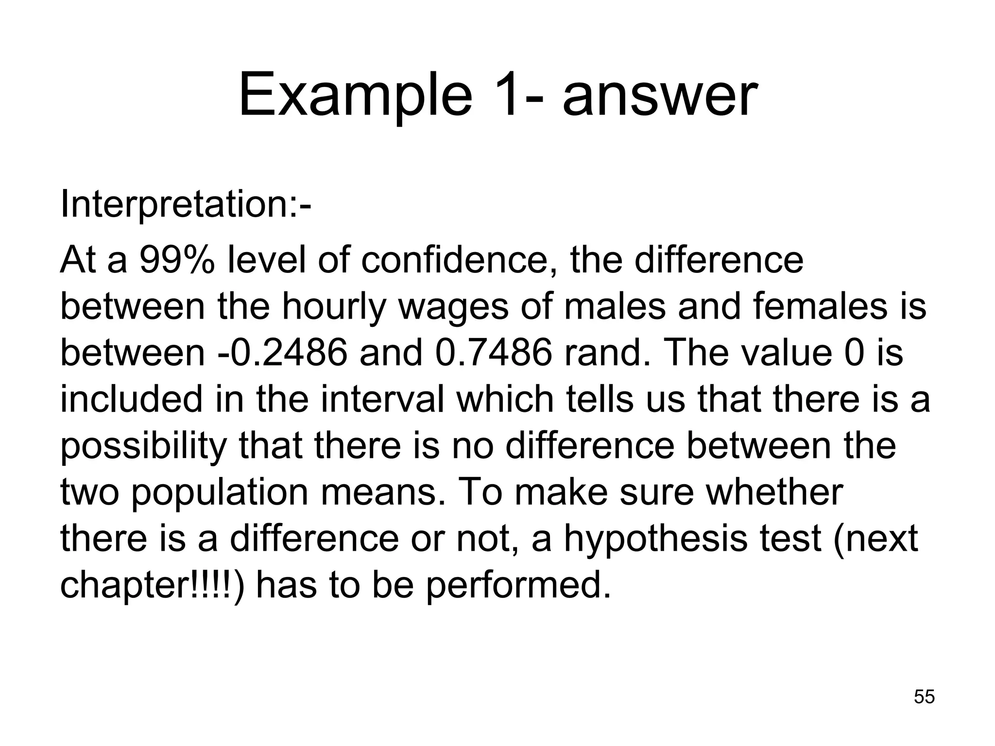
54. Example 1- Answer
 0,01
1   0,99 1  1
2 2
  0,01
 0,995
Z 0,995= 2,57
 2 2 
CI(1 – 2 = 
)0,99  x1  x 2   Z  s1  s2 


1
2
n1 n 2 

 2 
 6  5,75  2,57 0,95  0,75 
2

=  
45 32 
  
= [–0,2486;0,7486] 54

55. Example 1- answer
Interpretation:-
At a 99% level of confidence, the difference
between the hourly wages of males and females is
between -0.2486 and 0.7486 rand. The value 0 is
included in the interval which tells us that there is a
possibility that there is no difference between the
two population means. To make sure whether
there is a difference or not, a hypothesis test (next
chapter!!!!) has to be performed.
55

56. • Confidence interval difference in means
– Small independent samples
– When sample sizes are small, n1 & n2< 30 we use
the t distribution
NOTE: If both the limits of the confidence interval are
negative you should suspect that the mean of first
population is smaller than mean of second population56

57. Example
A plant that operates two shifts per week would like to
consider the difference in productivity for the two shifts. The
number of units that each shift produces on each of the 5
working days is recorded in the following table:-
Monday Tuesday Wednesday Thursday Friday
Shift 1 263 288 290 275 255
Shift 2 265 278 277 268 244
Assuming that the number of units produced by each shift
is normally distributed and that the population standard
deviations for the two shifts are equal construct a 99%
confidence interval for the difference in mean productivity
for the two shifts and comment on the result. 57

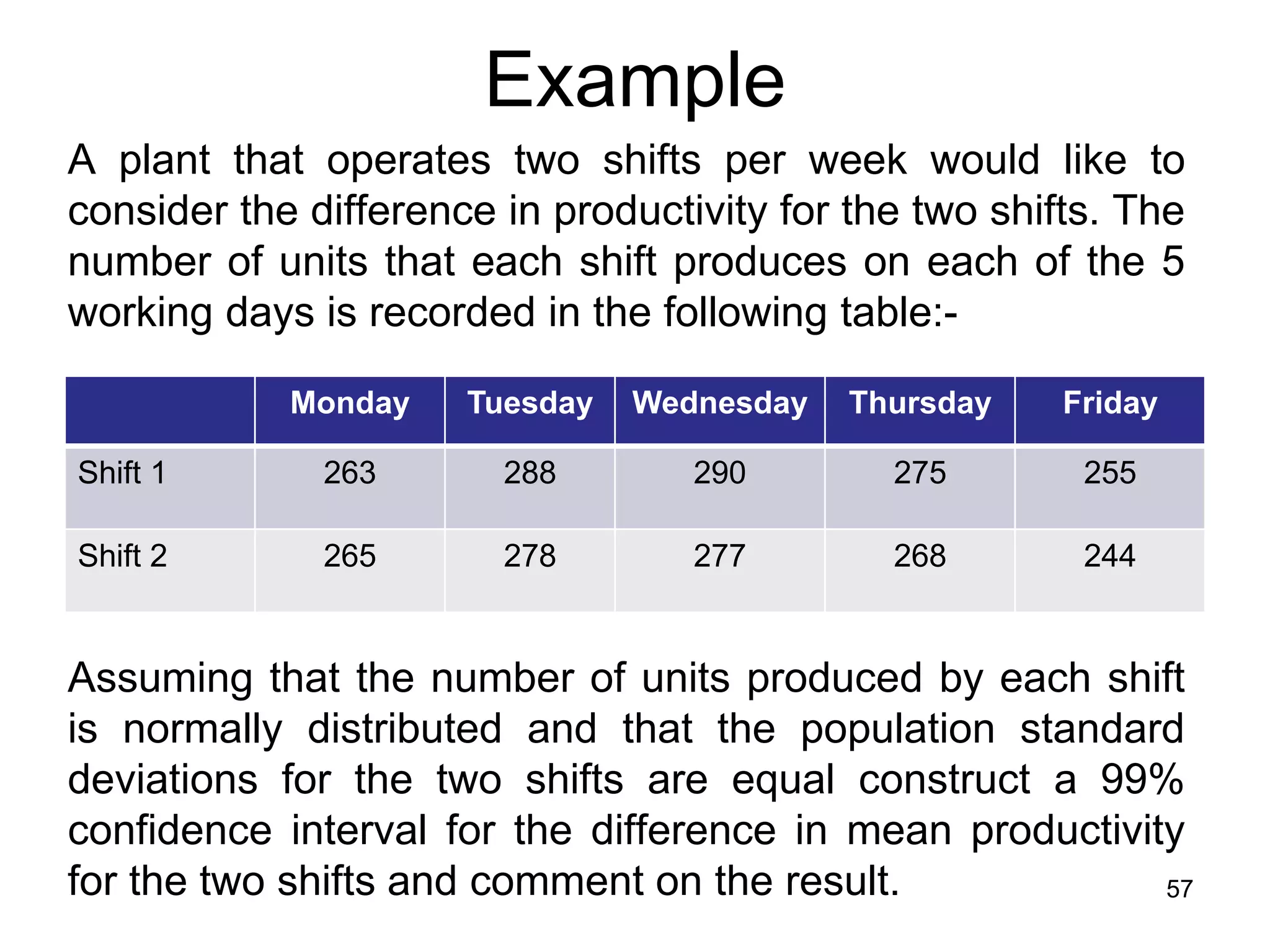
58. x
Example 1 - answer
 x2
1
x1  x2 
n1 n2
1 371 1 332
 
5 5
 274, 2  266, 4
     
1 2 1 2
2 2
x1  x1 x2  x2
2 n1 2 n2
s1  s2 
 n1 1
 n 2 1
 233,7  188,3
sp =
n1 1s12  n 2 1s2
2
n1  n 2  2
 
=
51(233,7)  51(188,3)
 5 5 2
 = 14,5258
 0,01
1   0,99 1  1
 2 2
  0,01
 0,995
t 8; 0,995 = 3,355
 1 1 
 CI(1 – 2 =  x1  x 2   t
)0,99   sp  

 n1 n 2 2;1
2
n1 n 2 


1 1
= [(274,2 – 266,4)  3,355(14,5258)  ]
5 5

= [–23,0221;38,6221]
At the 99% confidence level, because zero is included in the interval, it is possible that there
58

is no significant difference between the two shifts with respect to productivity.

59. CONCEPT QUESTIONS
• Nos 29 -39, p 235 – 237, textbook
59

60. • Confidence interval difference in
proportions
– Large independent samples
 p1 1  p1  p2 1  p2  
ˆ ˆ ˆ ˆ
CI ( p1  p2 )1   p1  p2   z1 
ˆ ˆ  


2 n1 n2 

x1 x2
with p1 
ˆ and p2 
ˆ
n1 n2
60

61. Example 1
Two groups of males are polled concerning
their interest in a new electric razor that has
four cutting edges. A sample of 64 males
under the age of 40 indicated that only 12
were interested while in a sample of 36
males over the age of 40, only 8 indicated
an interest. Construct a 95% confidence
interval for the difference between age froup
populations
61

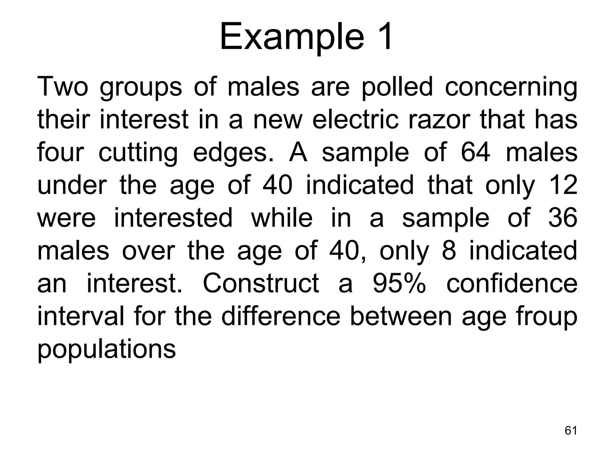
62. Example 1 - answer
12
ˆ
Under 40: n1 = 64 and p1 = = 0,1875.
64
8
ˆ
Over 40: n2 = 36 and p2 = = 0,2222.
36
1   0,95  1   1 0,05

2 2
  0,05

  0,975
Z 0,975 = 1,96
 p11 p1  p2 1 p2  
ˆ ˆ ˆ ˆ
CI( p1  p2 ) = 
0,9  p1  p2   Z 
ˆ ˆ + 


1
2
n1 n2 

 0,18750,8125 0,22220,7778 
=  0,1875 0,2222 1,96
  

 64 36 


= [–0,2008;0,1314]
62

63. • Confidence interval for the ratio of two population
variances
• We use the f distribution, table A5. See handout
 2  2 
 
 
2
CI   1  s1 
 2
1  ; s1 F 
 s2  F 

  1
2
  s2 2 n2 1; n1 1;
2
  n1 1; n2 1;
 
2
2
NOTE: If 1 does not lie in the confidence interval, there
is some evidence that the population variances are not
equal
63

64. EXAMPLE 1
A criminologist is interested in comparing the
consistency of the lengths of sentences given to
people convicted of robbery by two judges. A
random sample of 17 people convicted of robbery
by judge 1 showed a standard deviation of 2.53
years, while a random sample of 21 people
convicted by judge 2 showed a standard deviation
of 1.34 years. Construct a 95% confidence interval
for the ratio of the two populations variances. Does
the data suggest that the variances of the lengths
of sentences by the two judges differ? Motivate
your answer.
64

65. Example 1 - answer
Judge 1: n = 17 and s = 2,53.
1 1
Judge 2: n2 = 21 and s2 = 1,34.
 0,05
1   0,95 
2 2
  0,05
 0,025
F  = F16; 20; 0,025
n1 1;n 2 1;
2
 = 2,55
F   = F20; 16; 0,025
n 2 1;n1 1;
2
= 2,68
   
 s 2   s 2  

 12 1 1 
 
1
CI( 2 )0,95 =  2   2 F
; 
2 F n 2 1; n1 1; 
s2  n 1;n 1;  s2  2 
  1 2
2  
 2,53 2 
  1  2,53 2,68 
2
2 
=  2 
;

 1,34 2,55  1,34
 


= [1,3979;9,5536]
Yes, at the 95% level of confidence it is possible that the variances differ because 1 is not
65

included in the interval.

66. CONCEPT QUESTIONS
• Concept questions 40 – 47, p 241,
textbook
66

67. DETERMINING SAMPLE
SIZES FOR ESTIMATES
• Everything we have done so far has assumed
that a sample has ALREADY been taken
• We often need to know how large a sample
should we take to construct the confidence
interval
• Many factors can affect sample size such as
budget, time and ease of selection
• We will now look at how to determine the proper
sample size (from a statistical perspective)
67

68. • Sample size for estimating means
– Confidence level (1 – α)
– Accepted sampling error - e
– Need to know σ, else use s
 z1  
2
n 
 e 
NOTE: Sample size, n, is required to be a whole
number. Therefore always round UP to the next
largest integer
68

69. EXAMPLE 1
A pharmaceutical company is considering a
request to pay for the continuing education
of its research scientists. It would like to
estimate the average amount spent by these
scientists for professional memberships.
Base on a pilot study the standard deviation
is estimated to be R35. If a 95% confidence
of being correct to within +/- R20 is desired,
what sample size is necessary?
69

70. Example 1 - answer
 = 35 e = 20
 0,05
1   0,95 1  1
2 2
  0,05
 0,975
Z 0,975 = 1,96
2
Z   
 1 2 

n = 
 e 
 
2
1,9635 

=  
 20 

= 11,7649  12
At least 12 scientists should be selected. 70


71. • Sample size for estimating
proportions
– Confidence level (1 – α)
– Accepted sampling error - e
– Need to know p, else use p ˆ
2
 z1 
n  p (1  p )
 e 
71

72. Example 1
An audit test to establish the % of
occurrence of failures to follow a specific
internal control procedure is to be
undertaken. The auditor decides that the
maximum tolerable error rate that is
permissible is 5%. What sample size is
necessary to achieve a sample precision of
+/- 0.02 with 99% confidence?
72

73. Example 1 - answer
p = 0,05
e = 0,02
 0,01
1   0,99 1  1
2 2
  0,01
 0,995
Z 0,995 = 2,57
2
Z  
  1 2 
p 1 p
n =    
  e 
 
2
2,57 
=   0,050,95
0,02 
 = 784,3319  785
A sample size of at least 785 is required. 73


74. Classwork
• Questions 48 – 52, pages 244 – 245 ,
textbook
• Self review test, p245, text book
• Izimvo Exchange 1 and 2
• Activity 1,2,3
• Revision Exercise 1,2,3 and 4
74

75. HOMEWORK
• Supplementary questions, p249 – 253,
textbook
75