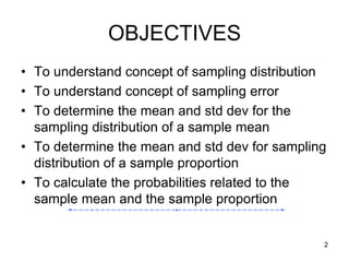
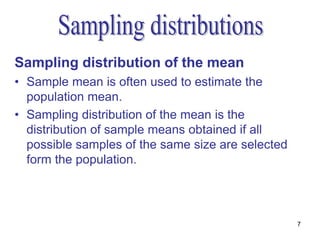
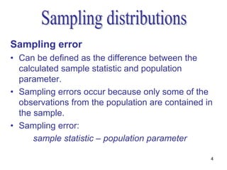
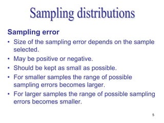
This document provides an overview of sampling distributions and sampling error. It aims to explain the concepts of the sampling distribution of the mean and proportion. Key points include: - Sampling distributions describe the distribution of sample statistics from repeated samples of a population. - Sampling error is the difference between a sample statistic and the population parameter. It depends on the sample size and decreases with larger samples. 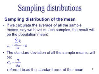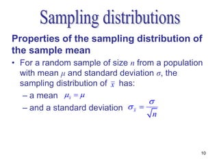- The sampling distribution of the mean for samples of size n from a normal population is a normal distribution with mean equal to the population mean and standard deviation equal to the population standard deviation divided by the square root of the sample size. 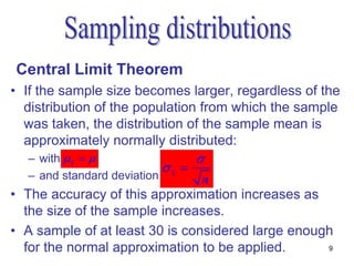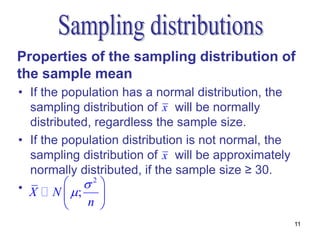- For sample sizes greater than 30, the Central Limit Theorem states the sampling

1. 1

2. OBJECTIVES
• To understand concept of sampling distribution
• To understand concept of sampling error
• To determine the mean and std dev for the
sampling distribution of a sample mean
• To determine the mean and std dev for sampling
distribution of a sample proportion
• To calculate the probabilities related to the
sample mean and the sample proportion
2

3. Sampling distributions
• Can be defined as the distribution of a sample
statistic.
• Scientific experiments are used to make
inferences concerning population parameters from
sample statistics.
• Need to know what is the relationship between the
sample statistic and its corresponding population
parameter.
3

4. Sampling error
• Can be defined as the difference between the
calculated sample statistic and population
parameter.
• Sampling errors occur because only some of the
observations from the population are contained in
the sample.
• Sampling error:
sample statistic – population parameter
4

5. Sampling error
• Size of the sampling error depends on the sample
selected.
• May be positive or negative.
• Should be kept as small as possible.
• For smaller samples the range of possible
sampling errors becomes larger.
• For larger samples the range of possible sampling
errors becomes smaller.
5

6. CONCEPT QUESTIONS
• P201 QUESTIONS 1-4
6

7. Sampling distribution of the mean
• Sample mean is often used to estimate the
population mean.
• Sampling distribution of the mean is the
distribution of sample means obtained if all
possible samples of the same size are selected
form the population.
7

8. Sampling distribution of the mean
• If we calculate the average of all the sample
means, say we have m such samples, the result will
be the population mean:
m
x i
x  i 1

m
• The standard deviation of all the sample means, will
be:

x 
n
referred to as the standard error of the mean 8

9. Central Limit Theorem
• If the sample size becomes larger, regardless of the
distribution of the population from which the sample
was taken, the distribution of the sample mean is
approximately normally distributed:
– with  x   
x 
– and standard deviation n
• The accuracy of this approximation increases as
the size of the sample increases.
• A sample of at least 30 is considered large enough
for the normal approximation to be applied. 9

10. Properties of the sampling distribution of
the sample mean
• For a random sample of size n from a population
with mean μ and standard deviation σ, the
sampling distribution of x has:
– a mean  x  

– and a standard deviation  x 
n
10

11. Properties of the sampling distribution of
the sample mean
• If the population has a normal distribution, the
sampling distribution of x will be normally
distributed, regardless the sample size.
• If the population distribution is not normal, the
sampling distribution of x will be approximately
normally distributed, if the sample size ≥ 30.
• X N ;  2 
 
 n 
11

12. Example
• Marks for a semester test is normally distributed,
with a mean of 60 and a standard deviation of 8.
– X ~ N(60;82)
• A sample of 25 students is randomly selected:

– X N  x ; x 2 
 2   82 
X N ;   N  60; 
 n   25 
12

13. Example
• If we need to determine the probability that the
average mark for the 25 students will be between
58 and 63.
P (58  X  63)
 
 58  60 63  60 
 P Z 
 8 8 
 
 25 25 
 P  1, 25  Z  1,88 
 0,9699  0,8944  1  0,8643

14. INDIVIDUAL EXERCISE
14

15. INDIVIDUAL EXERCISE
The past sales record for ice cream indicates
the sales are right skewed, with the
population mean of R13.50 per customer
and a std dev of R6.50. A random sample of
100 sales records is selected. Find the
probability of:-
1. Getting a mean of less than R13.25
2. Getting a mean of greater than R14.50
3. Getting a mean of between R13.80 and
R15.20
15

16. Solution
P205 - 207 of textbook
16

17. WHICH EQUATION TO USE?
17

18. Sampling distribution of
proportion
• Categorical values such as number of
drivers that wear safety belts in Gauteng
or number of drivers who do not wear
safety belts
18

19. Sampling distribution of the proportion
• Population proportion will be represented by p,
and the sample proportion by p  X / n, where X is
ˆ
the number of items with the characteristic and n
is the sample size.
• The standard error of the proportion is given as:
p(1  p)
p 
n
19

20. Example
• Suppose that in a class of 100, 28 students fail a
test.
• The population proportion of students who fail the
test is:
X 28
p 
ˆ  0, 28
n 100
20

21. Example
• A sample of 50 students is randomly chosen
• What is the probability that more than 25% will fail
the test?
ˆ
P P  0, 25 
 
 0, 25  0, 28 
 PZ  
 0, 28(1  0, 28) 
 
 50 
 P  Z  0, 47 
 1  0, 6808  0,3192 21

22. Individual exercise/homework
• Read pages 195 – 211
• Self review test p 209
• Supplementary exercises p209
• Go to www.jillmitchell.net and view the following:-
• Video on sampling distributions
• Video on example of sampling distribution
• Video on central limit theorem
• Completely re-do the NUBE test using your textbook to
assist you.
22