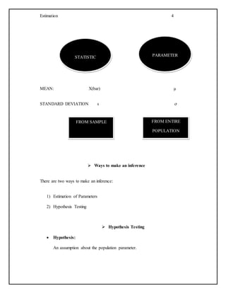
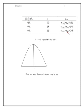
This document discusses key concepts in statistical estimation including: - Estimation involves using sample data to infer properties of the population by calculating point estimates and interval estimates. - A point estimate is a single value that estimates an unknown population parameter, while an interval estimate provides a range of plausible values for the parameter. - A confidence interval gives the probability that the interval calculated from the sample data contains the true population parameter. Common confidence intervals are 95% confidence intervals. 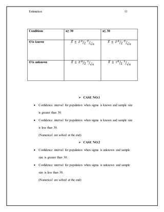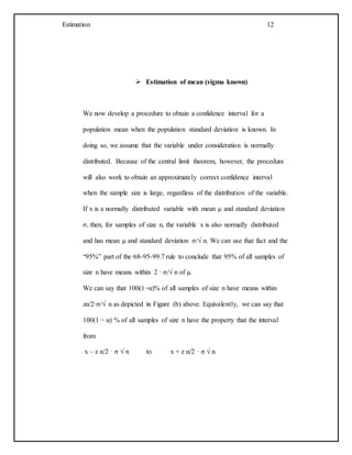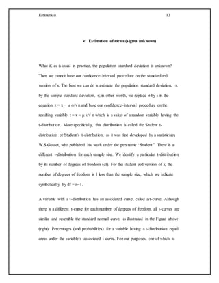- Formulas for confidence intervals depend on whether the population standard deviation is known or unknown, and the sample size.

1. Running Head: ESTIMATION 1
ESTIMATION

2. Estimation 2
Table of Contents
1. What is Inferential Statistics?
2. Ways to make an inference.
3. Estimation
4. Point Estimate
5. Interval Estimate
6. Confidence Interval
7. Cases.
8. Estimation of Mean (Sigma known)
9. Estimation of Mean (Sigma unknown)
10. Benefits of Estimation.
11. Drawbacks of Estimation.
12. Solved Numerical.

3. Estimation 3
 Inferential Statistics
Inferential statistics makes inferences about populations using data drawn from
the population. Instead of using the entire population to gather the data, the
statistician will collect a sample or samples from the millions of residents and
make inferences about the entire population using the sample.
Inferential statistical analysis infers properties about a population this includes
testing hypotheses and deriving estimates. The population is assumed to be larger
than the observed data set; in other words, the observed data is assumed to
be sampled from a larger population
Inferential statistics provide a way forgoing from a “sample” to a “population”
Inferring the “parameters” of a population from data on the “statistics” of a
sample .
 Parameter:
The numbers that describe the characteristics of the population(mean, sd,
variance etc)
 Statistics:
The numbers that describe characteristics of scores in the sample (mean,
Variance, s.d., correlation coefficient etc .)

4. Estimation 4
MEAN: X(bar) µ
STANDARD DEVIATION s ơ
 Ways to make an inference
There are two ways to make an inference:
1) Estimation of Parameters
2) Hypothesis Testing
 Hypothesis Testing
 Hypothesis:
An assumption about the population parameter.
STATISTIC PARAMETER
FROM SAMPLE FROM ENTIRE
POPULATION

5. Estimation 5
E.g. I assume the mean SBP of population is 120 mmHg
Hypothesis testing is an inferential procedure that uses sample data to evaluate the
credibility of a hypothesis about a population.
 Estimation
The process by which one makes inferences about a population, based on
information obtained from a sample.
Estimation statistics is a data analysis framework that uses a combination of
effect sizes confidence intervals, precision planning and meta-analysis to plan
experiments, analyze data and interpret results. It is distinct from null hypothesis
significance testing (NHST), which is considered to be less
informative. Estimation statistics, or simply estimation, is also known as the new
statistics, a distinction introduced in the fields of psychology, medical research,
life sciences and a wide range of other experimental sciences where NHST still
remains prevalent, despite estimation statistics having been recommended as
preferable for several decades.[The primary aim of estimation methods is to
estimate the size of an effect and report an effect size along with its confidence
intervals, the latter of which is related to the precision of the estimate. Estimation
at its core involves analyzing data to obtain a point estimate (an effect

6. Estimation 6
size calculated from data used as estimate of the population effect size) and
an interval estimate that summarizes a range of likely values of the underlying
population effect. Proponents of estimation see reporting a p-value as an
unhelpful distraction from the important business of reporting an effect size with
its confidence intervals, and believe that estimation should replace significance
testing for data analysis.
 Point Estimate:
Point estimates are single points that estimates parameter directly which
serve as a "best guess" or "best estimate" of an unknown population
parameter.
 Sample proportion pˆ(“p hat”) is the point estimate of p
 Sample mean x (“x bar”) is the point estimate of μ
 Sample standard deviation s is the point estimate of σ
 Interval Estimate:
Interval estimation is the use of sample data to calculate an interval of plausible
values of an unknown population parameter this is in contrast to point estimation.
We estimate an interval of statistics within which the population parameter
may be expected to lie with a certain degree of confidence.

7. Estimation 7
 Formula for Interval of Statistics
𝑋̅ ± 𝑍 𝛼
2⁄ 𝜎
√𝑛⁄
This formula has been derived from normal distribution.
 Upper Limit:
𝑋̅ − 𝑍 𝛼
2⁄ 𝜎
√𝑛⁄
 Lower Limit:
𝑋̅ + 𝑍 𝛼
2⁄ 𝜎
√𝑛⁄
 Confidence Interval
Confidence Interval is the probability that the interval computed from the sample
data includes the population parameter of interest.
Arrange of values used to estimate a population parameter is known as Interval
estimation or estimation by confidence and the interval a,b that will include the
population parameter with a high probability is known as confidence interval.
Confidence interval for a population mean (called a Z-interval)

8. Estimation 8
CONFIDENCE INTERVAL = 𝑿̅ ± (𝒁 𝟏 − 𝜶
𝟐)⁄
 The “α” level represents the “lack of confidence”
 (1−α) 100% represent the confidence level of a confidence interval
 Z(1-α/2) instead of z(1-α) in this formula is because the random error
(imprecision) is split between right and left tail
CONFIDENCE INTERVAL

9. Estimation 9
 Z values for different confidence level Area under the curve

10. Estimation 10
 Total area under the curve
1
Total area under the curve is always equal to one.

11. Estimation 11
Conditions n≥ 30 n≤ 30
Ơ is known 𝑋̅ ± 𝑍 𝛼
2⁄ 𝜎
√𝑛⁄ 𝑋̅ ± 𝑍 𝛼
2⁄ 𝜎
√𝑛⁄
Ơ is unknown 𝑋̅ ± 𝑍 𝛼
2⁄ 𝑠
√𝑛⁄ 𝑋̅ ± 𝑡 𝛼
2⁄ 𝑠
√𝑛⁄
 CASE NO.1
 Confidence interval for population when sigma is known and sample size
is greater than 30.
 Confidence interval for population when sigma is known and sample size
is less than 30.
(Numerical are solved at the end)
 CASE NO.2
 Confidence interval for population when sigma is unknown and sample
size is greater than 30.
 Confidence interval for population when sigma is unknown and sample
size is less than 30.
(Numerical are solved at the end)

12. Estimation 12
 Estimation of mean (sigma known)
We now develop a procedure to obtain a confidence interval for a
population mean when the population standard deviation is known. In
doing so, we assume that the variable under consideration is normally
distributed. Because of the central limit theorem, however, the procedure
will also work to obtain an approximately correct confidence interval
when the sample size is large, regardless of the distribution of the variable.
If x is a normally distributed variable with mean µ and standard deviation
σ, then, for samples of size n, the variable x is also normally distributed
and has mean µ and standard deviation σ/√ n. We can use that fact and the
“95%” part of the 68-95-99.7 rule to conclude that 95% of all samples of
size n have means within 2 · σ/√ n of µ.
We can say that 100(1−α)% of all samples of size n have means within
zα/2·σ/√ n as depicted in Figure (b) above. Equivalently, we can say that
100(1 − α) % of all samples of size n have the property that the interval
from
x – z α/2 · σ √ n to x + z α/2 · σ √ n

13. Estimation 13
 Estimation of mean (sigma unknown)
What if, as is usual in practice, the population standard deviation is unknown?
Then we cannot base our confidence-interval procedure on the standardized
version of x. The best we can do is estimate the population standard deviation, σ,
by the sample standard deviation, s; in other words, we replace σ by s in the
equation z = x − µ σ/√ n and base our confidence-interval procedure on the
resulting variable t = x − µ s/√ n which is a value of a random variable having the
t-distribution. More specifically, this distribution is called the Student t-
distribution or Student’s t-distribution, as it was first developed by a statistician,
W.S.Gosset, who published his work under the pen name “Student.” There is a
different t-distribution for each sample size. We identify a particular t-distribution
by its number of degrees of freedom (df). For the student zed version of x, the
number of degrees of freedom is 1 less than the sample size, which we indicate
symbolically by df = n−1.
A variable with a t-distribution has an associated curve, called a t-curve. Although
there is a different t-curve for each number of degrees of freedom, all t-curves are
similar and resemble the standard normal curve, as illustrated in the Figure above
(right). Percentages (and probabilities) for a variable having a t-distribution equal
areas under the variable’s associated t-curve. For our purposes, one of which is

14. Estimation 14
obtaining confidence intervals for a population mean, we don’t need a complete t-
table for each t-curve; only certain areas will be important.
 Flaws in hypothesis testing
In hypothesis testing, the primary objective of statistical calculations is to obtain
a p-value, the probability of seeing an obtained result, or a more extreme result,
when assuming the null hypothesis is true. If the p-value is low (usually < 0.05),
the statistical practitioner is then encouraged to reject the null hypothesis.
Proponents of estimation reject the validity of hypothesis testing for the
following reasons, among others:
 P-values are easily and commonly misinterpreted. For example, the p-value is
often mistakenly thought of as 'the probability that the null hypothesis is true.'
 The null hypothesis is always wrong for every set of observations: there is
always some effect, even if it is minuscule.
 Hypothesis testing produces arbitrarily dichotomous yes-no answers, while
discarding important information about magnitude.
 Any particular p-value arises through the interaction of the effect size,
the sample size (all things being equal a larger sample size produces a smaller
p-value) and sampling error.

15. Estimation 15
 At low power, simulation reveals that sampling error makes p-values
extremely volatile.
 Benefits of Estimation
 Advantages of confidence intervals:
Confidence intervals behave in a predictable way. By definition, 95%
confidence intervals have a 95% chance of capturing the underlying
population mean (μ). This feature remains constant with increasing sample
size; what changes is that the interval becomes smaller (more precise). In
addition, 95% confidence intervals are also 83% prediction intervals: one
experiment's confidence intervals have an 83% chance of capturing any
other future experiment's mean. As such, knowing a single experiment's
95% confidence intervals give the analyst a plausible range for the
population mean and plausible outcomes of any subsequent replication
experiments.
 Evidence based statistics
Psychological studies of the perception of statistics reveal that reporting
interval estimates leaves a more accurate perception of the data than
reporting p-values.

16. Estimation 16
 Precision planning
The precision of an estimate is formally defined as 1/variance, and like
power, increases (improves) with increasing sample size. Like power, a
high level of precision is expensive; research grant applications would
ideally include precision/cost analyses. Proponents of estimation believe
precision planning should replace power since statistical power itself is
conceptually linked to significance testing.

17. Estimation 17
Bibliography
Estimation definition,Benefits,Drawbacks,estimation of mean. (n.d.). Retrieved
from Wikipedia: https://en.wikipedia.org/wiki/Estimation_statistics
Flaws of Hypothesis testing. (n.d.). Retrieved from statistics show to.:
www.statisticshowto.com/probability-and-statistics/hypothesis-testing/
Inferential Statistics. (n.d.). Retrieved from Study.com:
study.com/academy/lesson/descriptive-and-inferential-statistics.html