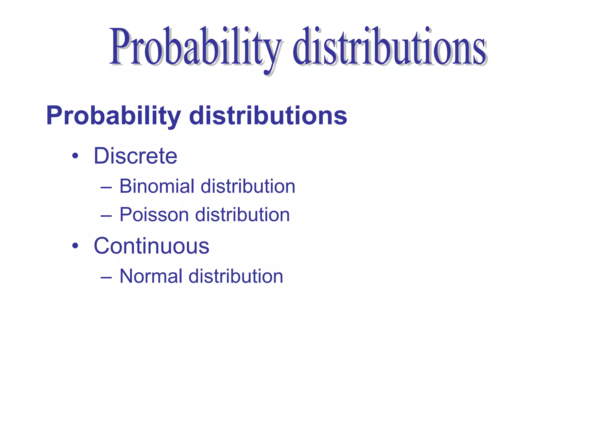
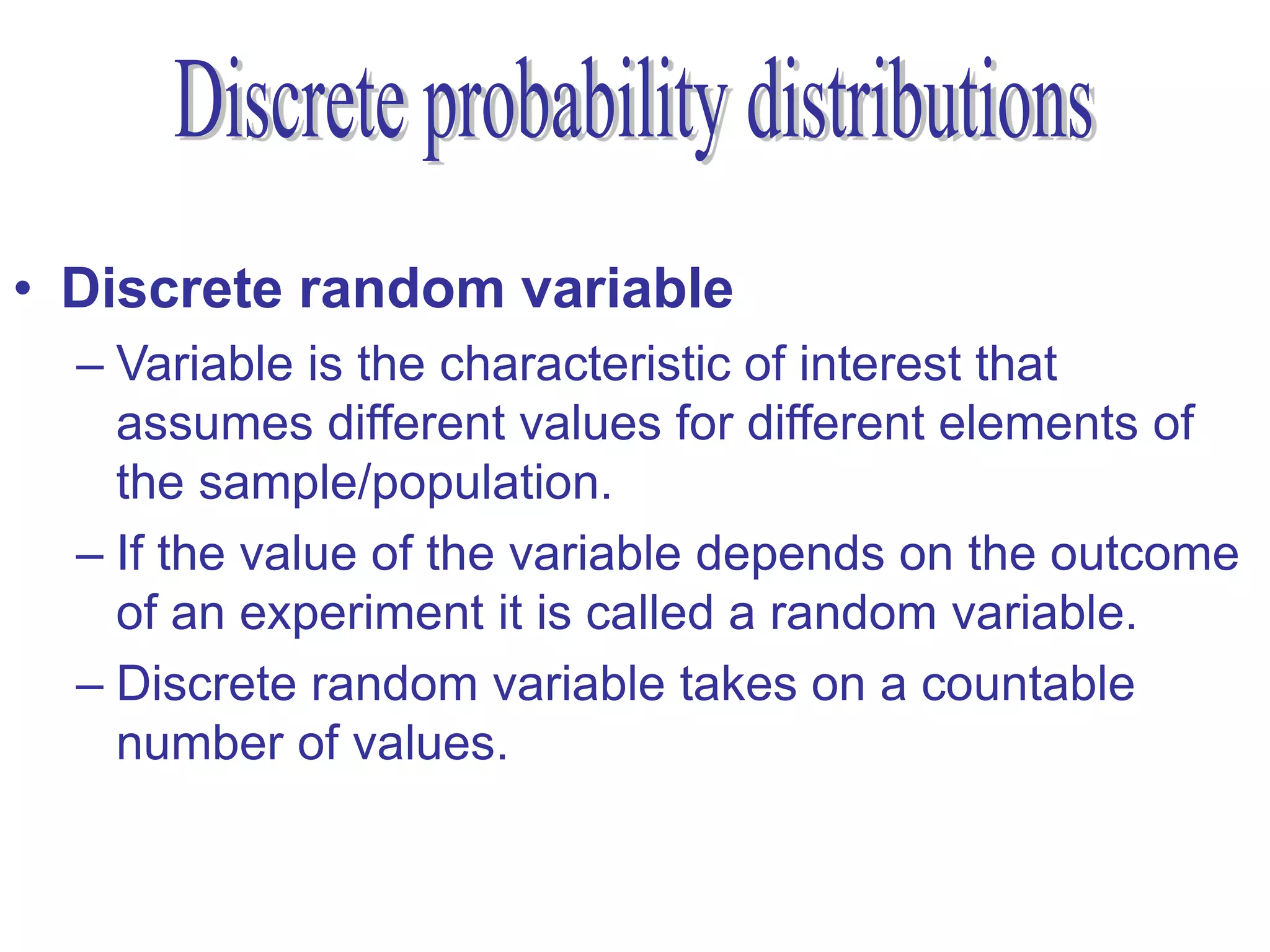
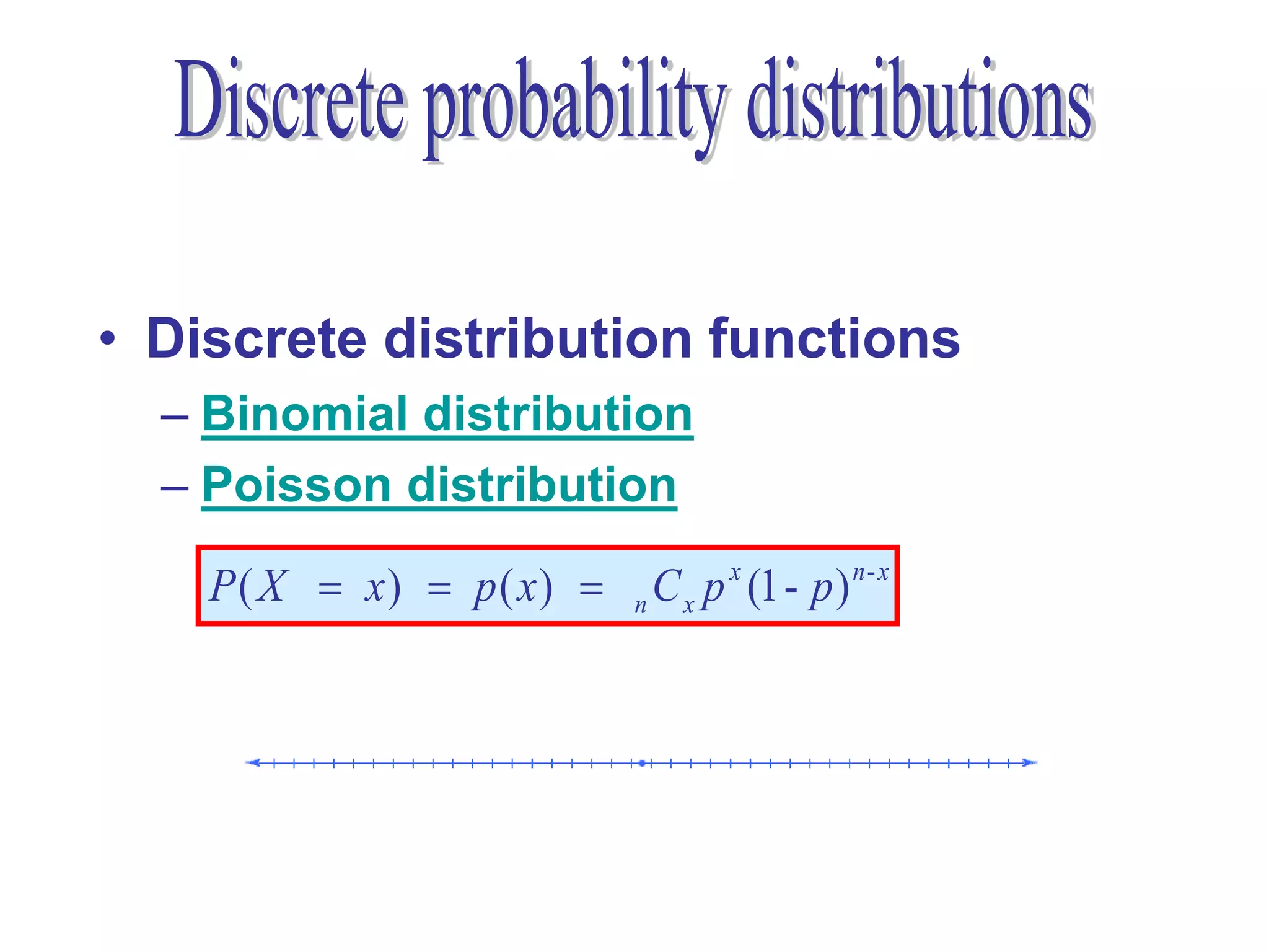
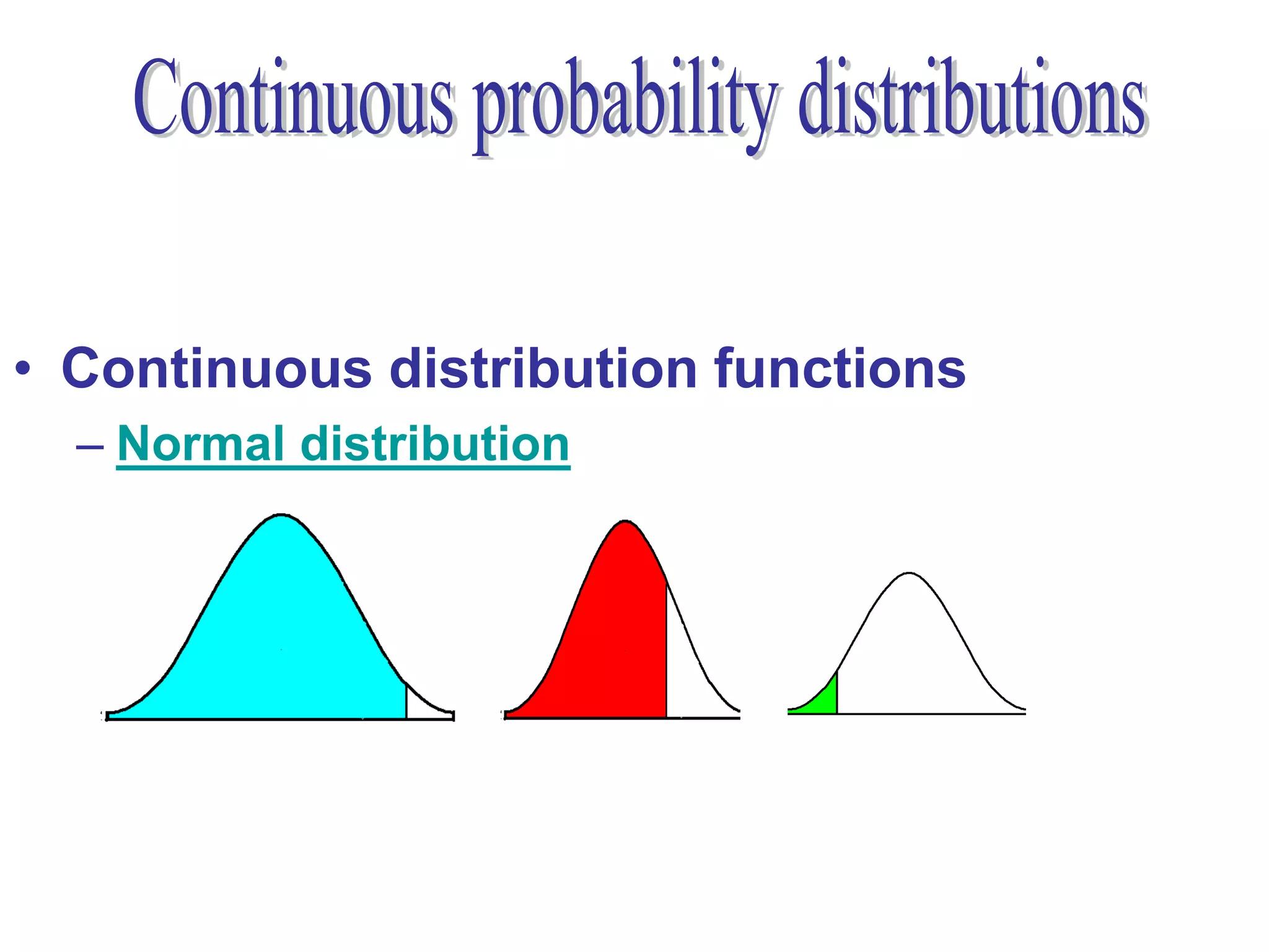
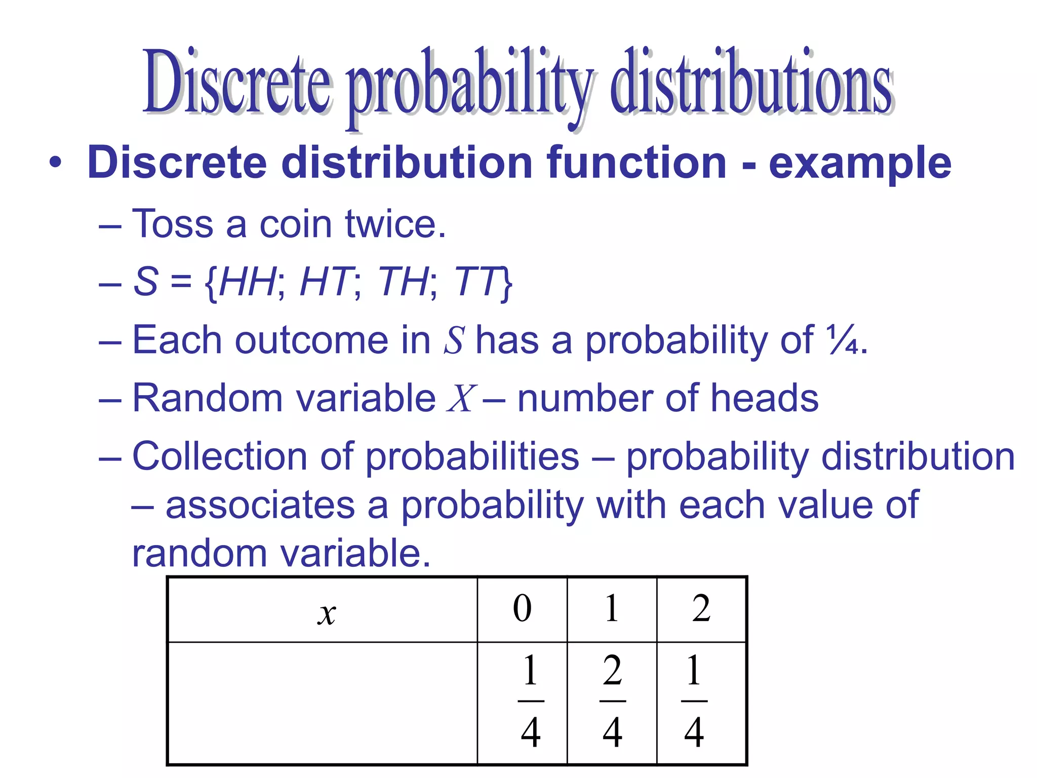
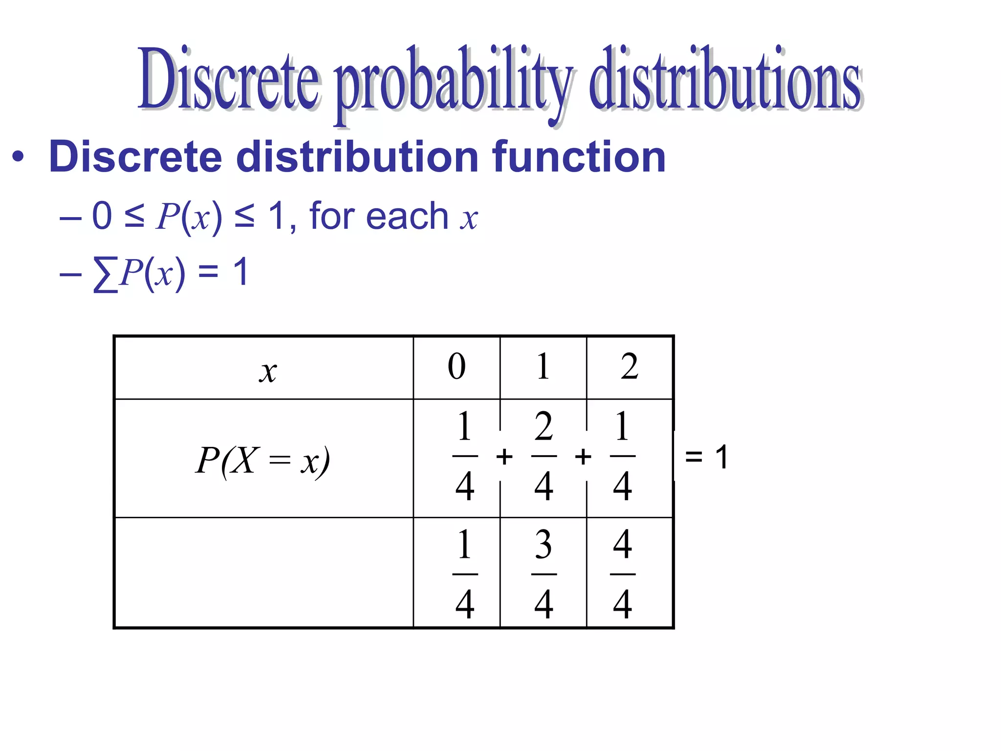
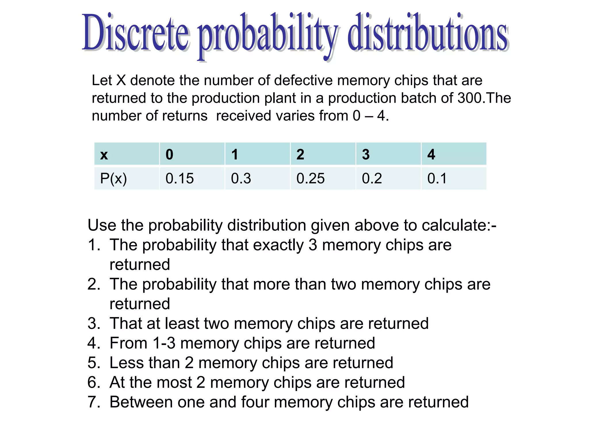
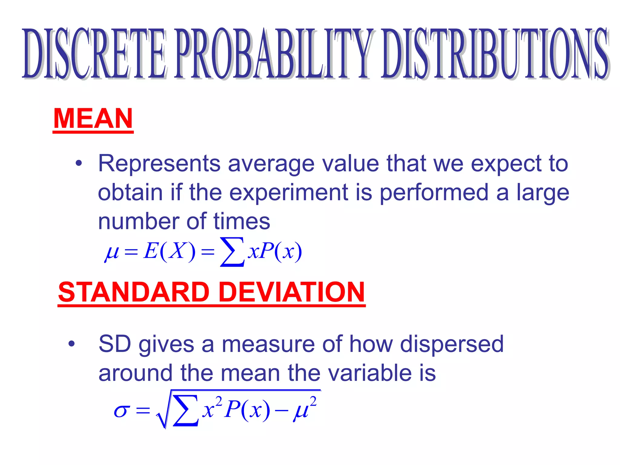
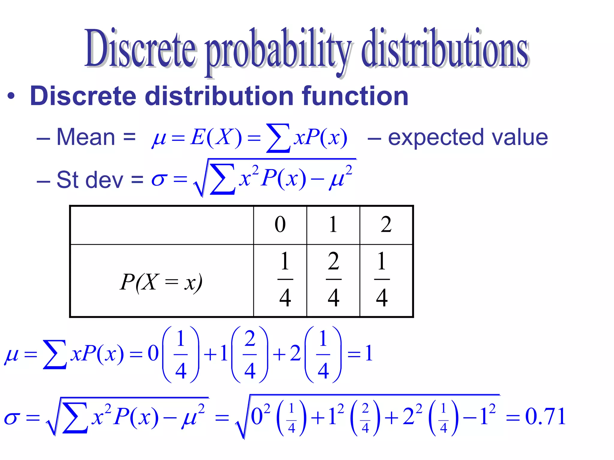
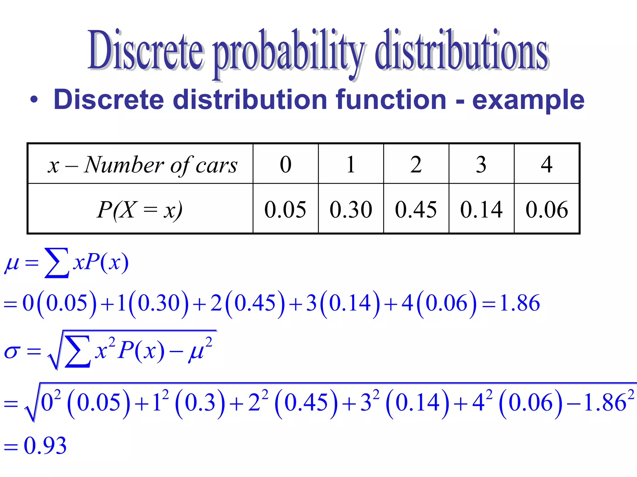
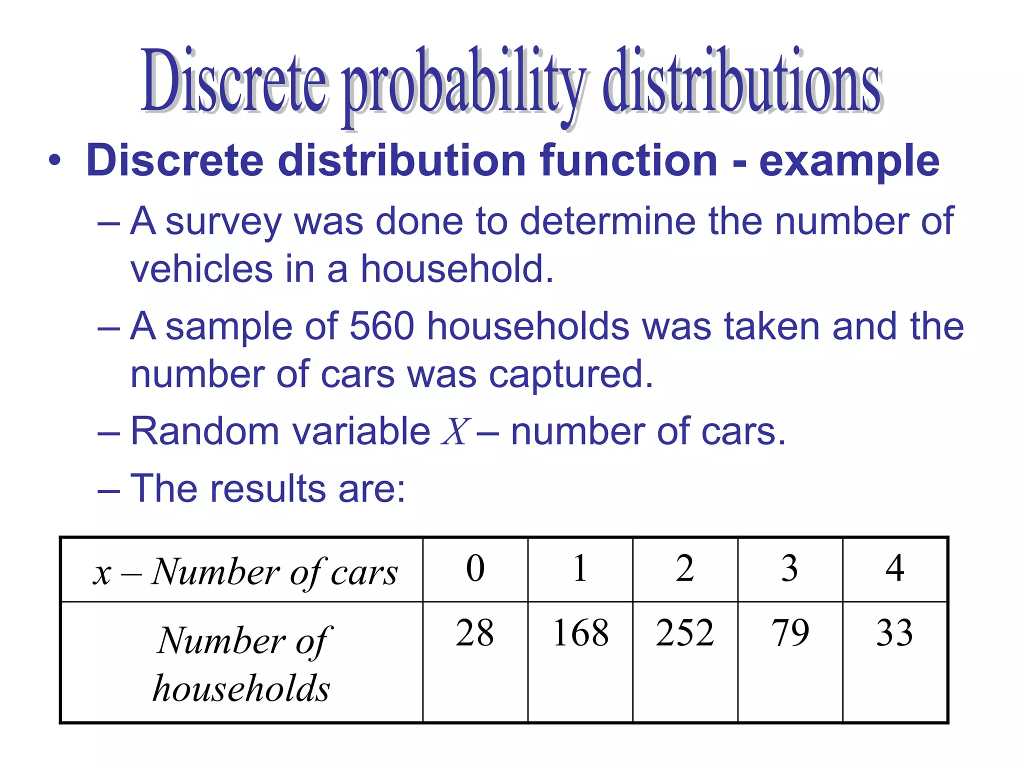
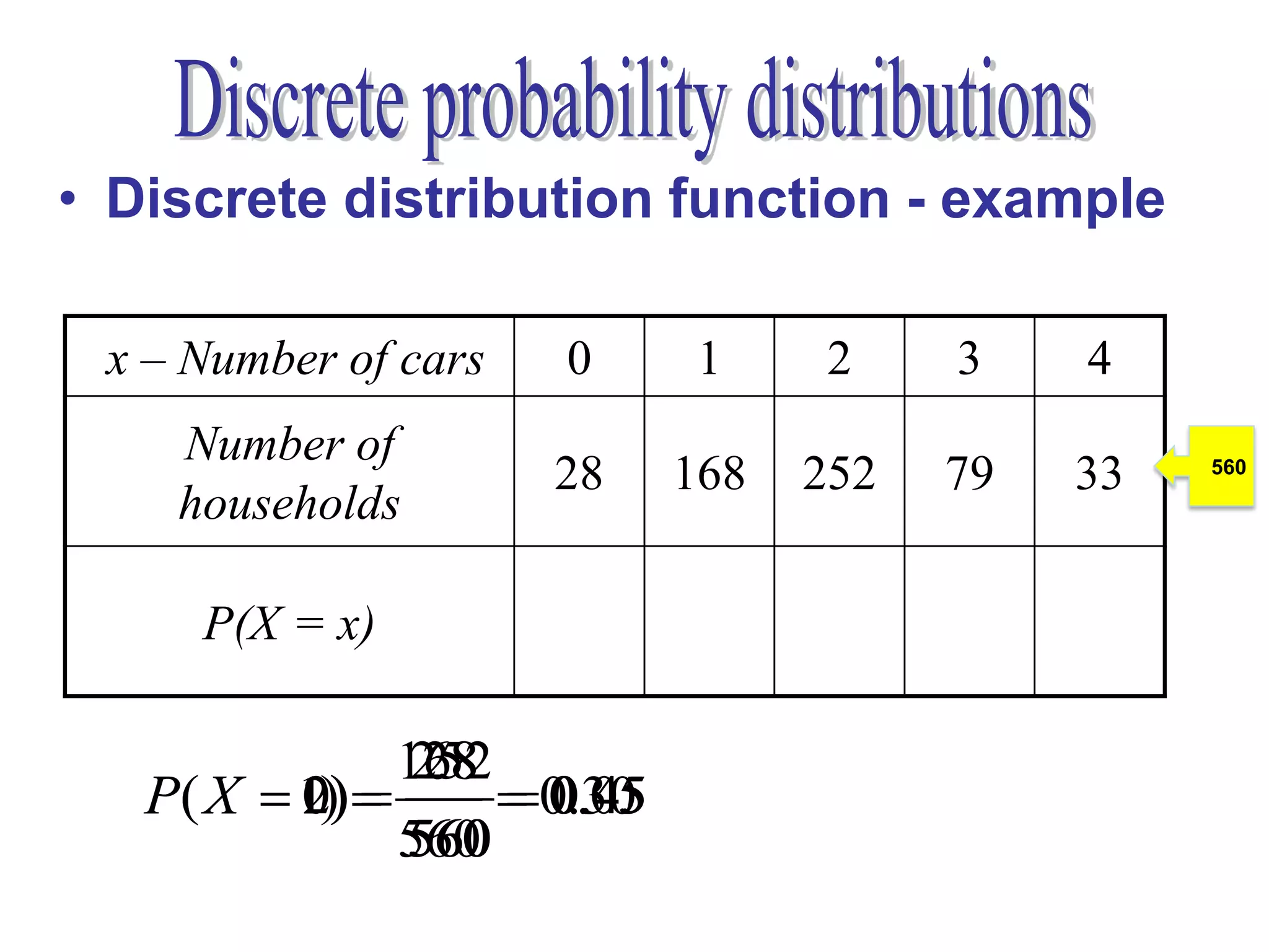
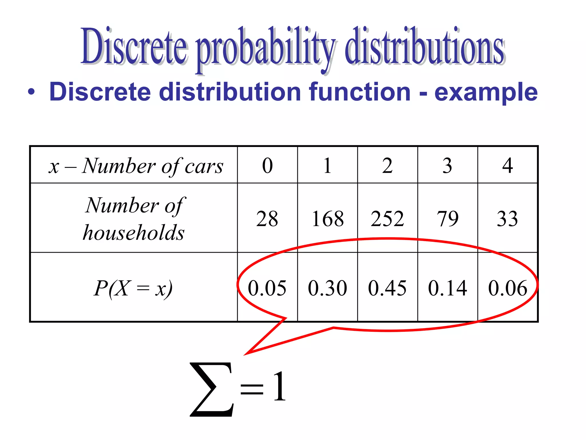
This document discusses probability distributions and some key concepts: 1. It describes discrete and continuous random variables and examples like the binomial, Poisson, and normal distributions. 2. For discrete random variables, it explains how to calculate probabilities, mean, and standard deviation from a probability distribution table. 3. An example is provided to demonstrate calculating these values from data on the number of vehicles owned by households. 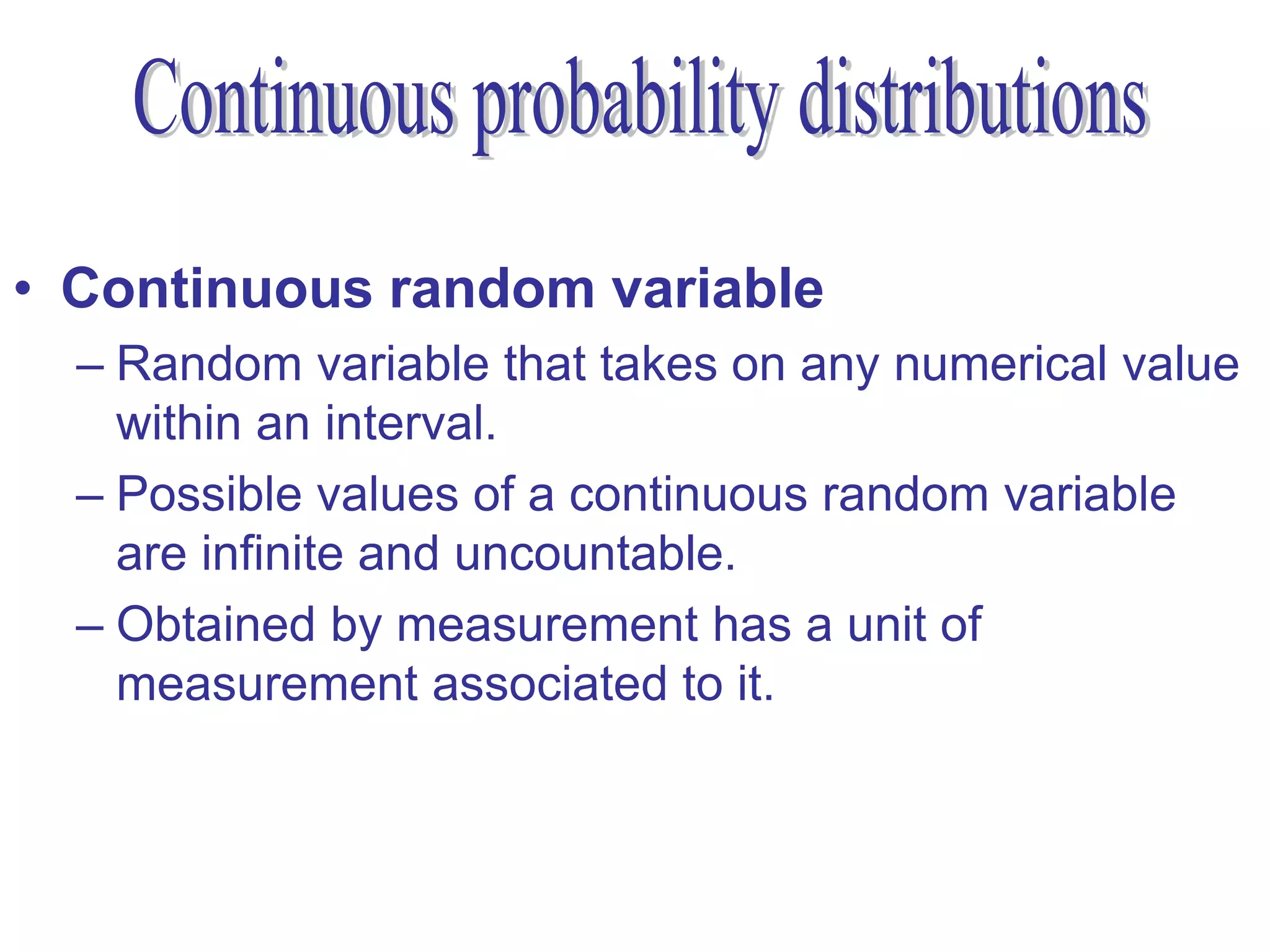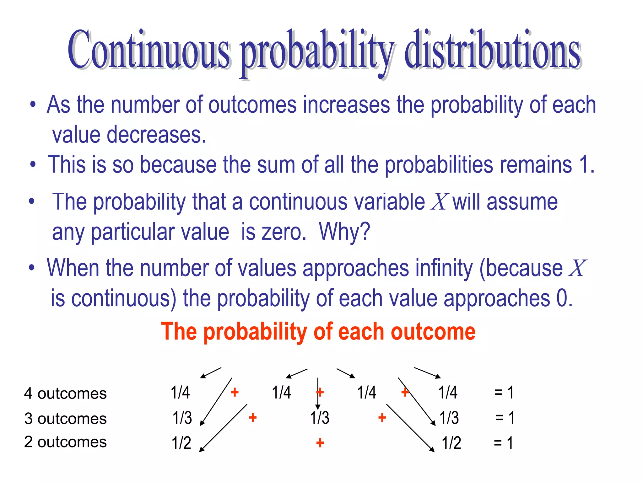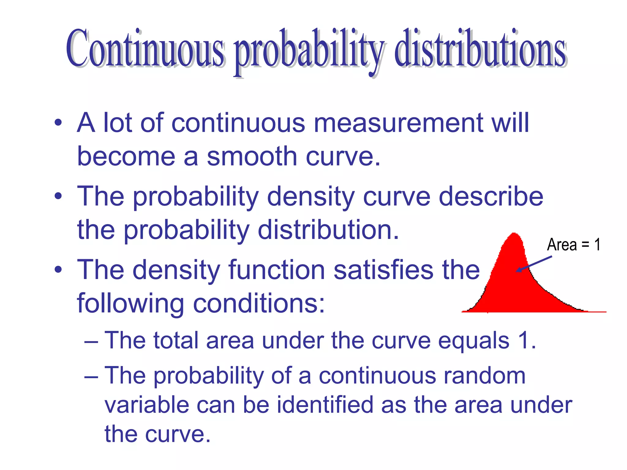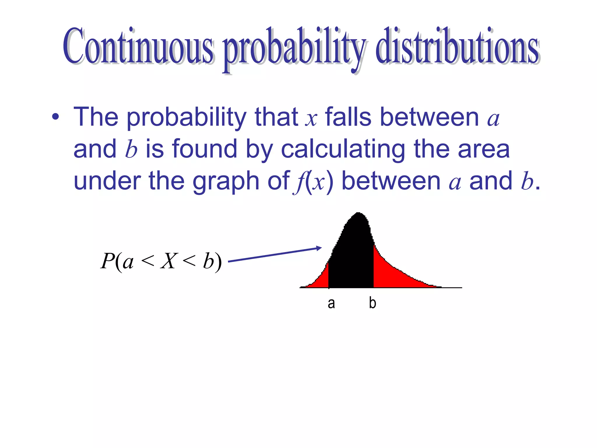4. It also introduces continuous random variables and density functions, noting that the probability of any single value is zero due to the infinite number of possible outcomes. The area under the density function curve represents probabilities.

2. Probability distributions
• Discrete
– Binomial distribution
– Poisson distribution
• Continuous
– Normal distribution

3. • Discrete random variable
– Variable is the characteristic of interest that
assumes different values for different elements of
the sample/population.
– If the value of the variable depends on the outcome
of an experiment it is called a random variable.
– Discrete random variable takes on a countable
number of values.

4. • Discrete distribution function - example
– Toss a coin twice.
– S = {HH; HT; TH; TT}
– Each outcome in S has a probability of ¼.
– Random variable X – number of heads
– Collection of probabilities – probability distribution
– associates a probability with each value of
random variable.
x 0 1 2
1 2 1
P(X = x) = P(x)
4 4 4

5. • Discrete distribution function
– 0 ≤ P(x) ≤ 1, for each x
– ∑P(x) = 1
x 0 1 2
1 2 1
P(X = x) + + =1
4 4 4
1 3 4
P(X ≤ x)
4 4 4

6. Let X denote the number of defective memory chips that are
returned to the production plant in a production batch of 300.The
number of returns received varies from 0 – 4.
x 0 1 2 3 4
P(x) 0.15 0.3 0.25 0.2 0.1
Use the probability distribution given above to calculate:-
1. The probability that exactly 3 memory chips are
returned
2. The probability that more than two memory chips are
returned
3. That at least two memory chips are returned
4. From 1-3 memory chips are returned
5. Less than 2 memory chips are returned
6. At the most 2 memory chips are returned
7. Between one and four memory chips are returned

7. Answers
• Example 5.3, p154 Elementary
Statistics

8. MEAN
• Represents average value that we expect to
obtain if the experiment is performed a large
number of times
  E ( X )   xP( x)
STANDARD DEVIATION
• SD gives a measure of how dispersed
around the mean the variable is
   x P( x)  
2 2

9. • Discrete distribution function
– Mean =   E ( X )   xP( x) – expected value
– St dev =    x 2 P( x)   2
0 1 2
1 2 1
P(X = x)
4 4 4
1 2 1
   xP( x)  0    1   2    1
4 4 4
  x 2 P( x)   2  02  1
4
 12 
2
4
 22 
1
4
 12  0.71

10. • Discrete distribution function - example
– A survey was done to determine the number of
vehicles in a household.
– A sample of 560 households was taken and the
number of cars was captured.
– Random variable X – number of cars.
– The results are:
x – Number of cars 0 1 2 3 4
Number of 28 168 252 79 33
households

11. • Discrete distribution function - example
x – Number of cars 0 1 2 3 4
Number of
28 168 252 79 33 560
households
P(X = x) 0.05 0.30 0.45 0.14 0.06
252
28
168
P( X  1) 
0) 
2)  0.05
 0.30
0.45
560
560

12. • Discrete distribution function - example
x – Number of cars 0 1 2 3 4
Number of
28 168 252 79 33
households
P(X = x) 0.05 0.30 0.45 0.14 0.06
1

13. • Discrete distribution function - example
x – Number of cars 0 1 2 3 4
P(X = x) 0.05 0.30 0.45 0.14 0.06
   xP( x)
 0  0.05  1 0.30   2  0.45   3  0.14   4  0.06   1.86
  x 2 P( x)   2
 0  0.05   1  0.3  2  0.45   3  0.14   4  0.06   1.86
2 2 2 2 2 2
 0.93

14. • Discrete distribution functions
– Binomial distribution
– Poisson distribution
P( X  x)  p( x)  n C x p x (1- p ) n - x

15. • Continuous random variable
– Random variable that takes on any numerical value
within an interval.
– Possible values of a continuous random variable
are infinite and uncountable.
– Obtained by measurement has a unit of
measurement associated to it.

16. •• Ascontinuous random variable has probability of each
A the number of outcomes increases the an uncountable
value decreases.
infinite number of values in the interval (a,b)
• This is so because the sum of all the probabilities remains 1.
• The probability that a continuous variable X will assume
any particular value is zero. Why?
• When the number of values approaches infinity (because X
is continuous) the probability of each value approaches 0.
The probability of each outcome
4 outcomes 1/4 + 1/4 + 1/4 + 1/4 =1
3 outcomes 1/3 + 1/3 + 1/3 =1
2 outcomes 1/2 + 1/2 =1

17. • A lot of continuous measurement will
become a smooth curve.
• The probability density curve describe
the probability distribution. Area = 1
• The density function satisfies the
following conditions:
– The total area under the curve equals 1.
– The probability of a continuous random
variable can be identified as the area under
the curve.

18. • The probability that x falls between a
and b is found by calculating the area
under the graph of f(x) between a and b.
P(a < X < b)
a b

19. • Continuous distribution functions
– Normal distribution