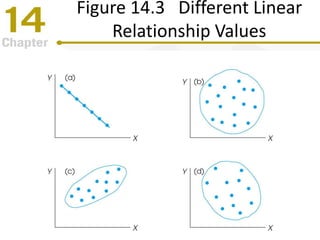
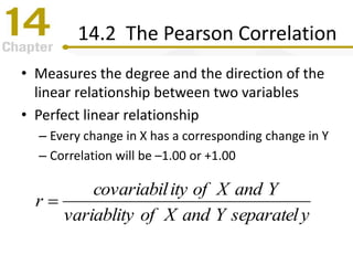
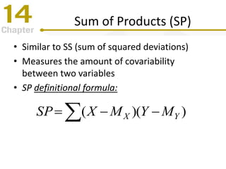
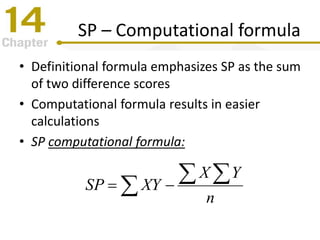
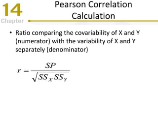
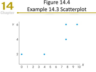
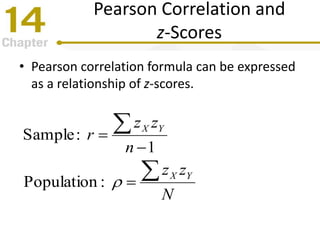
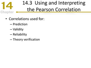
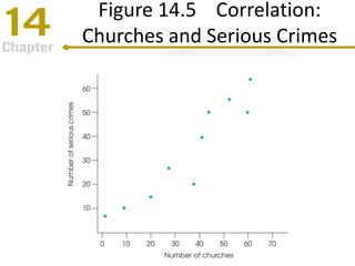
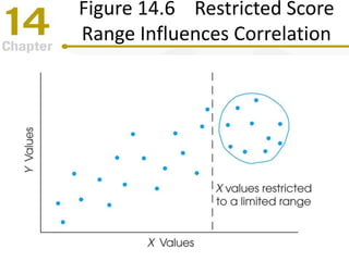
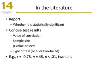
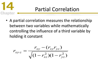
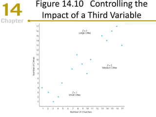
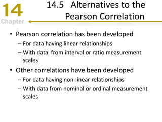
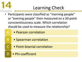
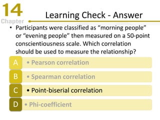
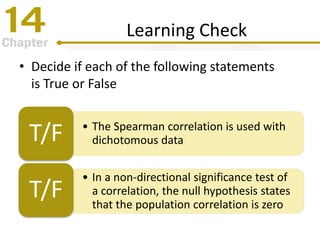
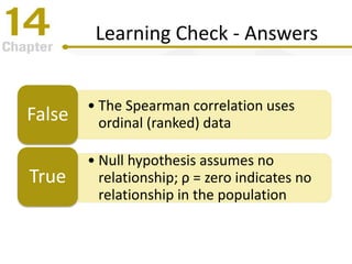
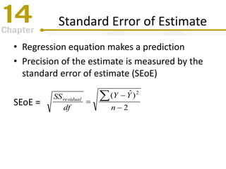
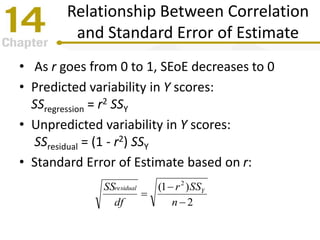
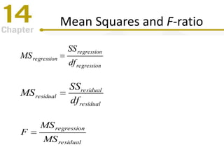
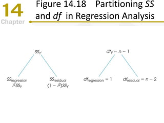
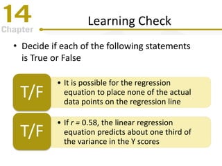
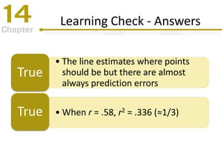
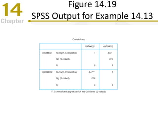
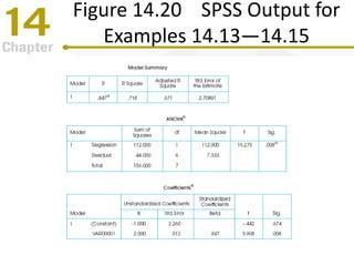
Chapter 14
Correlation and Regression
PowerPoint Lecture Slides
Essentials of Statistics for the
Behavioral Sciences
Eighth Edition
by Frederick J. Gravetter and Larry B. Wallnau
Chapter 14 Learning Outcomes
• Understand Pearson r as measure of variables’ relationship1
• Compute Pearson r using definitional or computational formula2
• Use and interpret Pearson r; understand assumptions &
limitations3
• Test hypothesis about population correlation (ρ) with sample r4
• Understand the concept of a partial correlation5
Chapter 14 Learning Outcomes
(continued)
• Explain/compute Spearman correlation coefficient (ranks)6
• Explain/compute point-biserial correlation coefficient (one
dichotomous variable)7
• Explain/compute phi-coefficient for two dichotomous variables8
• Explain/compute linear regression equation to predict Y values9
• Evaluate significance of regression equation10
Tools You Will Need
• Sum of squares (SS) (Chapter 4)
– Computational formula
– Definitional formula
• z-Scores (Chapter 5)
• Hypothesis testing (Chapter 8)
• Analysis of Variance (Chapter 12)
– MS values and F-ratios
14.1 Introduction to
Correlation
• Measures and describes the relationship
between two variables
• Characteristics of relationships
– Direction (negative or positive; indicated by the
sign, + or – of the correlation coefficient)
– Form (linear is most common)
– Strength or consistency (varies from 0 to 1)
• Characteristics are all independent
Figure 14.1 Scatterplot for
Correlational Data
Figure 14.2 Positive and
Negative Relationships
Figure 14.3 Different Linear
Relationship Values
14.2 The Pearson Correlation
• Measures the degree and the direction of the
linear relationship between two variables
• Perfect linear relationship
– Every change in X has a corresponding change in Y
– Correlation will be –1.00 or +1.00
yseparatelYandXofvariablity
YandXofitycovariabil
r 
Sum of Products (SP)
• Similar to SS (sum of squared deviations)
• Measures the amount of covariability
between two variables
• SP definitional formula:
  ))(( YX MYMXSP
SP – Computational formula
• Definitional formula emphasizes SP as the sum
of two difference scores
• Computational formula results in easier
calculations
• SP computational formula:
n
YX
XYSP
  
Pearson Correlation
Calculation
• Ratio comparing the covariability of X and Y
(numerator) with the variability of X and Y
separately (denominator)
YX SSSS
SP
r 
Figure 14.4
Example 14.3 Scatterplot
Pearson Correlation and
z-Scores
• Pearson correlation formula can be expressed
as a relationship of z-scores.
N
zz
n
zz
r
YX
YX





:Population
1
:Sample
Learning Check
• A scatterplot shows a set of data points that fit
very loosely around a line that slopes down to
the right. Which of the following values would
be closest to the correlation for these data?
• 0.75A
• 0.35B
• -0.75C
• -0.35D
Learning Check - Answer
• A scatterplot shows a set of data points that fit
very loosely around a line that slopes down to
the right. Which of the following values would
be closest to the correlation for these data?
• 0.75A
• 0.35B
• -0.75C
• -0.35D
Learning Check
• Decide if each of the following statements
is True or False
• A set of n = 10 pairs of X and Y
scores has ΣX = ΣY = ΣXY = 20.
For this set of scores, SP = –20
T/F
• If the Y variable decreases when
the X variable decreases, their
correlation is negative
T/F
Learning Check - Answers
204020
10
)20)(20(
20 SP
14.3 Using and Interpreting
the Pearson Correlation
• Correlations used for:
– Prediction
– Validity
– Reliability
– Theory verification
Interpreting Correlations
• Correlation describes a relationship but does
not demonstrate causation
• Establishing causation requires an experiment
in which one variable is manipulated and
others carefully controlled
• Example 14.4 (and Figure 14.5) demonstrates
the fallacy of attributing causation after
observing a correlation
Figure 14.5 Correlation:
Churches and Serious Crimes
Correlations and Restricted
Range of Scores
• Correlation coefficient value (size) will be
affected by the range of scores in the data
• Severely restricted range may provide a very
different correlation than would a broader
range of scores
• To be safe, never generalize a correlation
beyond the sample range of data
Figure 14.6 Restricted Score
Range Influences Correlation
Correlations and Outliers
• An outlier is an extremely deviant individual in
the sample
• Characterized by a much larger (or smaller)
score than all the others in the sample
• In a scatter plot, the point is clearly different
from all the other points
• Outliers produce a disproportionately large
impact on the correlation coefficient
Figure 14.7 Outlier Influences
Size of Correlation
Correlations and the Strength
of the Relationship
• A correlation coefficient measures the degree
of relationship on a scale from 0 to 1.00
• It is easy to mistakenly interpret this decimal
number as a percent or proportion
• Correlation is not a proportion
• Squared correlation may be interpreted as the
proportion of shared variability
• Squared correlation is called the coefficient of
determination
Coefficient of Determination
• Coefficient of determination measures the
proportion of variability in one variable that
can be determined from the relationship with
the other variable (shared variability)
2
rionDeterminatofoefficientC 
Figure 14.8 Three Amounts of
Linear Relationship Example
14.4 Hypothesis Tests with
the Pearson Correlation
• Pearson correlation is usually computed for
sample data, but used to test hypotheses
about the relationship in the population
• Population correlation shown by Greek letter
rho (ρ)
• Non-directional: H0: ρ = 0 and H1: ρ ≠ 0
Directional: H0: ρ ≤ 0 and H1: ρ > 0 or
Directional: H0: ρ ≥ 0 and H1: ρ < 0
Figure 14.9 Correlation in
Sample vs. Population
Correlation Hypothesis Test
• Sample correlation r used to test population ρ
• Degrees of freedom (df) = n – 2
• Hypothesis test can be computed using
either t or F; only t shown in this chapter
• Use t table to find critical value with df = n - 2
)2(
)1( 2




n
r
r
t

In the Literature
• Report
– Whether it is statistically significant
• Concise test results
– Value of correlation
– Sample size
– p-value or level
– Type of test (one- or two-tailed)
• E.g., r = -0.76, n = 48, p < .01, two tails
Partial Correlation
• A partial correlation measures the relationship
between two variables while mathematically
controlling the influence of a third variable by
holding it constant
)1)(1(
)(
22
yzxz
yzxyxy
zxy
rr
rrr
r



Figure 14.10 Controlling the
Impact of a Third Variable
14.5 Alternatives to the
Pearson Correlation
• Pearson correlation has been developed
– For data having linear relationships
– With data from interval or ratio measurement
scales
• Other correlations have been developed
– For data having non-linear relationships
– With data from nominal or ordinal measurement
scales
Spearman Correlation
• Spearman (rs) correlation formula is used with
data from an ordinal scale (ranks)
– Used when both variables are measured on an
ordinal scale
– Also may be used if measurement scales is interval
or ratio when relationship is consistently
directional but may not be linear
Figure 14.11 Consistent
Nonlinear Positive Relationship
Figure 14.12 Scatterplot
Showing Scores and Ranks
Ranking Tied Scores
• Tie scores need ranks for Spearman
correlation
• Method for assigning rank
– List scores in order from smallest to largest
– Assign a rank to each position in the list
– When two (or more) scores are tied, compute the
mean of their ranked position, and assign this
mean value as the final rank for each score.
Special Formula for the
Spearman Correlation
• The ranks for the scores are simply integers
• Calculations can be simplified
– Use D as the difference between the X rank and
the Y rank for each individual to compute the rs
statistic
)1(
6
1 2
2



nn
D
rs
Point-Biserial Correlation
• Measures relationship between two variables
– One variable has only two values
(called a dichotomous or binomial variable)
• Effect size for independent samples t-test in
Chapter 10 can be measures by r2
– Point-biserial r2 has same value as the r2
computed from t-statistic
– t-statistic tests significance of the mean difference
– r statistic measures the correlation size
Point-Biserial Correlation
• Applicable in the same situation as the
independent-measures t test in Chapter 10
– Code one group 0 and the other 1 (or any two
digits) as the Y score
– t-statistic evaluates the significance of mean
difference
– Point-Biserial r measures correlation magnitude
– r2 quantifies effect size
Phi Coefficient
• Both variables (X and Y) are dichotomous
– Both variables are re-coded to values 0 and 1 (or
any two digits)
– The regular Pearson formulas is used to calculate r
– r2 (coefficient of determination) measures effect
size (proportion of variability in one score
predicted by the other)
Learning Check
• Participants were classified as “morning people”
or “evening people” then measured on a 50-point
conscientiousness scale. Which correlation
should be used to measure the relationship?
• Pearson correlationA
• Spearman correlationB
• Point-biserial correlationC
• Phi-coefficientD
Learning Check - Answer
• Participants were classified as “morning people”
or “evening people” then measured on a 50-point
conscientiousness scale. Which correlation
should be used to measure the relationship?
• Pearson correlationA
• Spearman correlationB
• Point-biserial correlationC
• Phi-coefficientD
Learning Check
• Decide if each of the following statements
is True or False
• The Spearman correlation is used with
dichotomous dataT/F
• In a non-directional significance test of
a correlation, the null hypothesis states
that the population correlation is zero
T/F
Learning Check - Answers
• The Spearman correlation uses
ordinal (ranked) dataFalse
• Null hypothesis assumes no
relationship; ρ = zero indicates no
relationship in the population
True
14.6 Introduction to Linear
Equations and Regression
• The Pearson correlation measures a linear
relationship between two variables
• Figure 14.13 makes the relationship obvious
• The line through the data
– Makes the relationship easier to see
– Shows the central tendency of the relationship
– Can be used for prediction
• Regression analysis precisely defines the line
Figure 14.13 Regression line
Linear Equations
• General equation for a line
– Equation: Y = bX + a
– X and Y are variables
– a and b are fixed constant
Figure 14.14
Linear Equation Graph
Regression
• Regression is a method of finding an equation
describing the best-fitting line for a set of data
• How to define a “best fitting” straight line
when there are many possible straight lines?
• The answer: a line that is the best fit for the
actual data that minimizes prediction errors
Regression
• Ŷ is the value of Y predicted by the regression
equation (regression line) for each value of X
• (Y- Ŷ) is the distance each data point is from
the regression line: the error of prediction
• The regression procedure produces a line that
minimizes total squared error of prediction
• This method is called the least-squared-error
solution
Figure 14.15 Y-Ŷ Distance: Actual
Data Point Minus Predicted Point
Regression Equations
• Regression line equation: Ŷ = bX + a
• The slope of the line, b, can be calculated
• The line goes through (MX,MY) therefore
X
Y
X s
s
rb
SS
SP
b or 
XY bMMa 
Figure 14.16 Data Points and
Regression Line: Example 14.13
Standard Error of Estimate
• Regression equation makes a prediction
• Precision of the estimate is measured by the
standard error of estimate (SEoE)
SEoE = 2
)ˆ( 2




n
YY
df
SSresidual
Figure 14.17 Regression Lines:
Perfectly Fit vs. Example 14.13
Relationship Between Correlation
and Standard Error of Estimate
• As r goes from 0 to 1, SEoE decreases to 0
• Predicted variability in Y scores:
SSregression = r2 SSY
• Unpredicted variability in Y scores:
SSresidual = (1 - r2) SSY
• Standard Error of Estimate based on r:
2
)1( 2



n
SSr
df
SS Yresidual
Testing Regression Significance
• Analysis of Regression
– Similar to Analysis of Variance
– Uses an F-ratio of two Mean Square values
– Each MS is a SS divided by its df
• H0: the slope of the regression line (b or beta)
is zero
Mean Squares and F-ratio
residual
residual
residual
df
SS
MS 
regression
regression
regression
df
SS
MS 
residual
regression
MS
MS
F 
Figure 14.18 Partitioning SS
and df in Regression Analysis
Learning Check
• A linear regression has b = 3 and a = 4.
What is the “predicted Y” (Ŷ) for X = 7?
• 14A
• 25B
• 31C
• Cannot be determinedD
Learning Check - Answer
• A linear regression has b = 3 and a = 4.
What is the predicted Y for X = 7?
• 14A
• 25B
• 31C
• Cannot be determinedD
Learning Check
• Decide if each of the following statements
is True or False
• It is possible for the regression
equation to place none of the actual
data points on the regression line
T/F
• If r = 0.58, the linear regression
equation predicts about one third of
the variance in the Y scores
T/F
Learning Check - Answers
• The line estimates where points
should be but there are almost
always prediction errors
True
• When r = .58, r2 = .336 (≈1/3)True
Figure 14.19
SPSS Output for Example 14.13
Figure 14.20 SPSS Output for
Examples 14.13—14.15
Figure 14.21 Scatter Plot for
Data of Demonstration 14.1
Any
Questions
?
Concepts
?
Equations?

Correlation and Regression

  • 1.
    Chapter 14 Correlation andRegression PowerPoint Lecture Slides Essentials of Statistics for the Behavioral Sciences Eighth Edition by Frederick J. Gravetter and Larry B. Wallnau
  • 2.
    Chapter 14 LearningOutcomes • Understand Pearson r as measure of variables’ relationship1 • Compute Pearson r using definitional or computational formula2 • Use and interpret Pearson r; understand assumptions & limitations3 • Test hypothesis about population correlation (ρ) with sample r4 • Understand the concept of a partial correlation5
  • 3.
    Chapter 14 LearningOutcomes (continued) • Explain/compute Spearman correlation coefficient (ranks)6 • Explain/compute point-biserial correlation coefficient (one dichotomous variable)7 • Explain/compute phi-coefficient for two dichotomous variables8 • Explain/compute linear regression equation to predict Y values9 • Evaluate significance of regression equation10
  • 4.
    Tools You WillNeed • Sum of squares (SS) (Chapter 4) – Computational formula – Definitional formula • z-Scores (Chapter 5) • Hypothesis testing (Chapter 8) • Analysis of Variance (Chapter 12) – MS values and F-ratios
  • 5.
    14.1 Introduction to Correlation •Measures and describes the relationship between two variables • Characteristics of relationships – Direction (negative or positive; indicated by the sign, + or – of the correlation coefficient) – Form (linear is most common) – Strength or consistency (varies from 0 to 1) • Characteristics are all independent
  • 6.
    Figure 14.1 Scatterplotfor Correlational Data
  • 7.
    Figure 14.2 Positiveand Negative Relationships
  • 8.
    Figure 14.3 DifferentLinear Relationship Values
  • 9.
    14.2 The PearsonCorrelation • Measures the degree and the direction of the linear relationship between two variables • Perfect linear relationship – Every change in X has a corresponding change in Y – Correlation will be –1.00 or +1.00 yseparatelYandXofvariablity YandXofitycovariabil r 
  • 10.
    Sum of Products(SP) • Similar to SS (sum of squared deviations) • Measures the amount of covariability between two variables • SP definitional formula:   ))(( YX MYMXSP
  • 11.
    SP – Computationalformula • Definitional formula emphasizes SP as the sum of two difference scores • Computational formula results in easier calculations • SP computational formula: n YX XYSP   
  • 12.
    Pearson Correlation Calculation • Ratiocomparing the covariability of X and Y (numerator) with the variability of X and Y separately (denominator) YX SSSS SP r 
  • 13.
  • 14.
    Pearson Correlation and z-Scores •Pearson correlation formula can be expressed as a relationship of z-scores. N zz n zz r YX YX      :Population 1 :Sample
  • 15.
    Learning Check • Ascatterplot shows a set of data points that fit very loosely around a line that slopes down to the right. Which of the following values would be closest to the correlation for these data? • 0.75A • 0.35B • -0.75C • -0.35D
  • 16.
    Learning Check -Answer • A scatterplot shows a set of data points that fit very loosely around a line that slopes down to the right. Which of the following values would be closest to the correlation for these data? • 0.75A • 0.35B • -0.75C • -0.35D
  • 17.
    Learning Check • Decideif each of the following statements is True or False • A set of n = 10 pairs of X and Y scores has ΣX = ΣY = ΣXY = 20. For this set of scores, SP = –20 T/F • If the Y variable decreases when the X variable decreases, their correlation is negative T/F
  • 18.
    Learning Check -Answers 204020 10 )20)(20( 20 SP
  • 19.
    14.3 Using andInterpreting the Pearson Correlation • Correlations used for: – Prediction – Validity – Reliability – Theory verification
  • 20.
    Interpreting Correlations • Correlationdescribes a relationship but does not demonstrate causation • Establishing causation requires an experiment in which one variable is manipulated and others carefully controlled • Example 14.4 (and Figure 14.5) demonstrates the fallacy of attributing causation after observing a correlation
  • 21.
  • 22.
    Correlations and Restricted Rangeof Scores • Correlation coefficient value (size) will be affected by the range of scores in the data • Severely restricted range may provide a very different correlation than would a broader range of scores • To be safe, never generalize a correlation beyond the sample range of data
  • 23.
    Figure 14.6 RestrictedScore Range Influences Correlation
  • 24.
    Correlations and Outliers •An outlier is an extremely deviant individual in the sample • Characterized by a much larger (or smaller) score than all the others in the sample • In a scatter plot, the point is clearly different from all the other points • Outliers produce a disproportionately large impact on the correlation coefficient
  • 25.
    Figure 14.7 OutlierInfluences Size of Correlation
  • 26.
    Correlations and theStrength of the Relationship • A correlation coefficient measures the degree of relationship on a scale from 0 to 1.00 • It is easy to mistakenly interpret this decimal number as a percent or proportion • Correlation is not a proportion • Squared correlation may be interpreted as the proportion of shared variability • Squared correlation is called the coefficient of determination
  • 27.
    Coefficient of Determination •Coefficient of determination measures the proportion of variability in one variable that can be determined from the relationship with the other variable (shared variability) 2 rionDeterminatofoefficientC 
  • 28.
    Figure 14.8 ThreeAmounts of Linear Relationship Example
  • 29.
    14.4 Hypothesis Testswith the Pearson Correlation • Pearson correlation is usually computed for sample data, but used to test hypotheses about the relationship in the population • Population correlation shown by Greek letter rho (ρ) • Non-directional: H0: ρ = 0 and H1: ρ ≠ 0 Directional: H0: ρ ≤ 0 and H1: ρ > 0 or Directional: H0: ρ ≥ 0 and H1: ρ < 0
  • 30.
    Figure 14.9 Correlationin Sample vs. Population
  • 31.
    Correlation Hypothesis Test •Sample correlation r used to test population ρ • Degrees of freedom (df) = n – 2 • Hypothesis test can be computed using either t or F; only t shown in this chapter • Use t table to find critical value with df = n - 2 )2( )1( 2     n r r t 
  • 32.
    In the Literature •Report – Whether it is statistically significant • Concise test results – Value of correlation – Sample size – p-value or level – Type of test (one- or two-tailed) • E.g., r = -0.76, n = 48, p < .01, two tails
  • 33.
    Partial Correlation • Apartial correlation measures the relationship between two variables while mathematically controlling the influence of a third variable by holding it constant )1)(1( )( 22 yzxz yzxyxy zxy rr rrr r   
  • 34.
    Figure 14.10 Controllingthe Impact of a Third Variable
  • 35.
    14.5 Alternatives tothe Pearson Correlation • Pearson correlation has been developed – For data having linear relationships – With data from interval or ratio measurement scales • Other correlations have been developed – For data having non-linear relationships – With data from nominal or ordinal measurement scales
  • 36.
    Spearman Correlation • Spearman(rs) correlation formula is used with data from an ordinal scale (ranks) – Used when both variables are measured on an ordinal scale – Also may be used if measurement scales is interval or ratio when relationship is consistently directional but may not be linear
  • 37.
    Figure 14.11 Consistent NonlinearPositive Relationship
  • 38.
  • 39.
    Ranking Tied Scores •Tie scores need ranks for Spearman correlation • Method for assigning rank – List scores in order from smallest to largest – Assign a rank to each position in the list – When two (or more) scores are tied, compute the mean of their ranked position, and assign this mean value as the final rank for each score.
  • 40.
    Special Formula forthe Spearman Correlation • The ranks for the scores are simply integers • Calculations can be simplified – Use D as the difference between the X rank and the Y rank for each individual to compute the rs statistic )1( 6 1 2 2    nn D rs
  • 41.
    Point-Biserial Correlation • Measuresrelationship between two variables – One variable has only two values (called a dichotomous or binomial variable) • Effect size for independent samples t-test in Chapter 10 can be measures by r2 – Point-biserial r2 has same value as the r2 computed from t-statistic – t-statistic tests significance of the mean difference – r statistic measures the correlation size
  • 42.
    Point-Biserial Correlation • Applicablein the same situation as the independent-measures t test in Chapter 10 – Code one group 0 and the other 1 (or any two digits) as the Y score – t-statistic evaluates the significance of mean difference – Point-Biserial r measures correlation magnitude – r2 quantifies effect size
  • 43.
    Phi Coefficient • Bothvariables (X and Y) are dichotomous – Both variables are re-coded to values 0 and 1 (or any two digits) – The regular Pearson formulas is used to calculate r – r2 (coefficient of determination) measures effect size (proportion of variability in one score predicted by the other)
  • 44.
    Learning Check • Participantswere classified as “morning people” or “evening people” then measured on a 50-point conscientiousness scale. Which correlation should be used to measure the relationship? • Pearson correlationA • Spearman correlationB • Point-biserial correlationC • Phi-coefficientD
  • 45.
    Learning Check -Answer • Participants were classified as “morning people” or “evening people” then measured on a 50-point conscientiousness scale. Which correlation should be used to measure the relationship? • Pearson correlationA • Spearman correlationB • Point-biserial correlationC • Phi-coefficientD
  • 46.
    Learning Check • Decideif each of the following statements is True or False • The Spearman correlation is used with dichotomous dataT/F • In a non-directional significance test of a correlation, the null hypothesis states that the population correlation is zero T/F
  • 47.
    Learning Check -Answers • The Spearman correlation uses ordinal (ranked) dataFalse • Null hypothesis assumes no relationship; ρ = zero indicates no relationship in the population True
  • 48.
    14.6 Introduction toLinear Equations and Regression • The Pearson correlation measures a linear relationship between two variables • Figure 14.13 makes the relationship obvious • The line through the data – Makes the relationship easier to see – Shows the central tendency of the relationship – Can be used for prediction • Regression analysis precisely defines the line
  • 49.
  • 50.
    Linear Equations • Generalequation for a line – Equation: Y = bX + a – X and Y are variables – a and b are fixed constant
  • 51.
  • 52.
    Regression • Regression isa method of finding an equation describing the best-fitting line for a set of data • How to define a “best fitting” straight line when there are many possible straight lines? • The answer: a line that is the best fit for the actual data that minimizes prediction errors
  • 53.
    Regression • Ŷ isthe value of Y predicted by the regression equation (regression line) for each value of X • (Y- Ŷ) is the distance each data point is from the regression line: the error of prediction • The regression procedure produces a line that minimizes total squared error of prediction • This method is called the least-squared-error solution
  • 54.
    Figure 14.15 Y-ŶDistance: Actual Data Point Minus Predicted Point
  • 55.
    Regression Equations • Regressionline equation: Ŷ = bX + a • The slope of the line, b, can be calculated • The line goes through (MX,MY) therefore X Y X s s rb SS SP b or  XY bMMa 
  • 56.
    Figure 14.16 DataPoints and Regression Line: Example 14.13
  • 57.
    Standard Error ofEstimate • Regression equation makes a prediction • Precision of the estimate is measured by the standard error of estimate (SEoE) SEoE = 2 )ˆ( 2     n YY df SSresidual
  • 58.
    Figure 14.17 RegressionLines: Perfectly Fit vs. Example 14.13
  • 59.
    Relationship Between Correlation andStandard Error of Estimate • As r goes from 0 to 1, SEoE decreases to 0 • Predicted variability in Y scores: SSregression = r2 SSY • Unpredicted variability in Y scores: SSresidual = (1 - r2) SSY • Standard Error of Estimate based on r: 2 )1( 2    n SSr df SS Yresidual
  • 60.
    Testing Regression Significance •Analysis of Regression – Similar to Analysis of Variance – Uses an F-ratio of two Mean Square values – Each MS is a SS divided by its df • H0: the slope of the regression line (b or beta) is zero
  • 61.
    Mean Squares andF-ratio residual residual residual df SS MS  regression regression regression df SS MS  residual regression MS MS F 
  • 62.
    Figure 14.18 PartitioningSS and df in Regression Analysis
  • 63.
    Learning Check • Alinear regression has b = 3 and a = 4. What is the “predicted Y” (Ŷ) for X = 7? • 14A • 25B • 31C • Cannot be determinedD
  • 64.
    Learning Check -Answer • A linear regression has b = 3 and a = 4. What is the predicted Y for X = 7? • 14A • 25B • 31C • Cannot be determinedD
  • 65.
    Learning Check • Decideif each of the following statements is True or False • It is possible for the regression equation to place none of the actual data points on the regression line T/F • If r = 0.58, the linear regression equation predicts about one third of the variance in the Y scores T/F
  • 66.
    Learning Check -Answers • The line estimates where points should be but there are almost always prediction errors True • When r = .58, r2 = .336 (≈1/3)True
  • 67.
    Figure 14.19 SPSS Outputfor Example 14.13
  • 68.
    Figure 14.20 SPSSOutput for Examples 14.13—14.15
  • 69.
    Figure 14.21 ScatterPlot for Data of Demonstration 14.1
  • 70.

Editor's Notes

  • #6 Instructors may wish to note that correlation coefficient cannot be smaller than -1 nor larger then +1. If calculation produce a number outside those boundaries, an error was made.
  • #7 FIGURE 14.1 Correlational data showing the relationship between family income (X) and student grades (Y) for a sample of n = 14 high school students. The scores are listed in order from lowest to highest family income and are shown in a scatter plot.
  • #8 FIGURE 14.2 Examples of positive and negative relationships. (a) Beer sales are positively related to temperature. (b) Coffee sales are negatively related to temperature.
  • #9 FIGURE 14.3 Examples of difference values for linear correlations: (a) a perfect negative correlation, -1.00; (b) no linear trend, 0.00; (c) a strong positive relationship, approximately +0.90; (d) a relatively weak negative correlation, approximately -0.40.
  • #14 FIGURE 14.4 Scatter plot of the data from Example 14.3.
  • #22 FIGURE 14.5 Hypothetical data showing the logical relationship between the number of churches and the number of serious crimes for a sample of U.S. cities.
  • #24 FIGURE 14.6 In this example, the full range of X and Y values shows a strong, positive correlation, but the restricted range of scores produces a correlation near zero.
  • #26 FIGURE 14.7 A demonstration of how one extreme data point (an outlier) can influence the value of a correlation.
  • #29 FIGURE 14.8 Three sets of data showing three different degrees of linear relationship.
  • #31 FIGURE 14.9 Scatter plot of a population of X and Y values with near-zero correlation. However, a small sample of n = 3 data points from this population shows a relatively strong, positive correlation. Data points in the sample are circled.
  • #35 FIGURE 14.10 Hypothetical data showing the relationship between the number of churches and the number of crimes for three groups of cities. Those with small populations (Z = 1), those with medium populations (Z = 2, and those with large populations (Z = 3).
  • #38 FIGURE 14.11 Hypothetical data showing the relationship between practice and performance. Although this relationship is not linear, there is a consistent positive relationship. An increase in performance tends to accompany an increase in practice.
  • #39 FIGURE 14.12 Scatter plots showing (a) the scores and (b) the ranks for the data in Example 15.9. Notice that there is a consistent, positive relationship between the X and Y scores, although it is not a linear relationship. Also, notice that the scatter plot of the ranks shows a perfect linear relationship.
  • #41 NOTE: This special formula is accurate ONLY when there are no tied ranks; as the number of tied ranks increases, the accuracy of the formula decreases. Also not that the value of the fraction has to be computed first, then subtracted from 1.
  • #50 FIGURE 14.13 Hypothetical data showing the relationship between SAT scores and GPA with a regression line drawn through the data points. The regression line defines a precise, one-to-one relationships between each X value (SAT score) and its corresponding Y value (GPA).
  • #52 FIGURE 14.14 The relationship between total cost and number of videos rented each month. The video store charges a $5 monthly membership fee and $2 for each video rented. The relationship is described by a linear equation, Y = 2X + 5, where Y is the total cost and X is the number of videos.
  • #55 FIGURE 14.15 The distance between the actual data points (Y) and the predicted point on the line (Ŷ) is defined as Y – Ŷ. The goal of regression is to find the equation for the line that minimizes these distances.
  • #57 FIGURE 14.16 The X and Y data points and the regression line for the n = 8 pairs of scores in Example 14.13.
  • #59 FIGURE 14.17 (a) A scatter plot showing data points that perfectly fit the regression line defined by the equation Ŷ = 2X – 1. Note that the correlation is r = +1.00. (b) A scatter plot for the data in Example 14.15. Notice that there is error between the actual data points and the predicted Y values on the regression line.
  • #63 FIGURE 14.18 The partitioning of SS and df for analysis of regression. The variability in the original Y scores (both SSY and dfY) is partitioned into two components: (1) the variability that is explained by the regression equation, and (2) the residual variability.
  • #68 FIGURE 14.19 The SPSS output showing the correlation for the data in Example 14.13.
  • #69 FIGURE 14.20 Portions of the SPSS output from the analysis of regression for the data in Examples 14.13, 14.14, and 14.15.
  • #70 FIGURE 14.21 The scatter plot for the data of Demonstration 14.1. An envelope is drawn around the points to estimate the magnitude of the correlation. A line is drawn through the middle of the envelope.