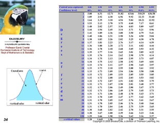
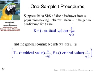
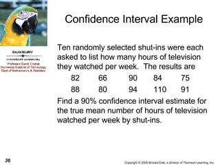
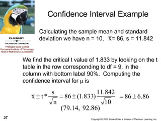
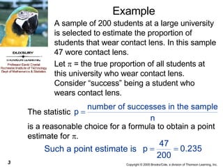
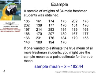
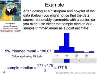
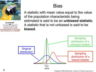
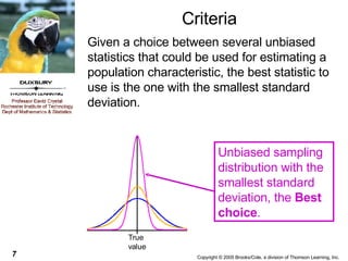
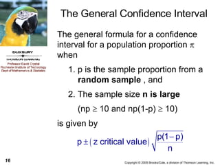
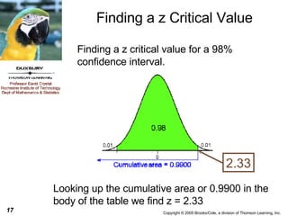
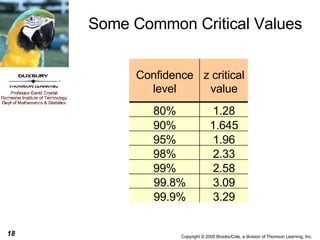
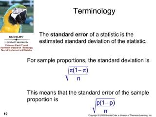
Chapter 9 Estimation Using a Single Sample
A  point estimate  of a population characteristic is a single number that is based on sample data and represents a plausible value of the characteristic. Point Estimation
Example A sample of 200 students at a large university is selected to estimate the proportion of students that wear contact lens. In this sample 47 wore contact lens. Let    = the true proportion of all students at this university who wear contact lens. Consider “success” being a student who wears contact lens.
Example A sample of weights of 34 male freshman students was obtained. 185 161 174 175 202 178 202 139 177 170 151 176 197 214 283 184 189 168 188 170 207 180 167 177  166 231 176 184 179 155 148 180 194 176 If one wanted to estimate the true mean of all male freshman students, you might use the sample mean as a point estimate for the true mean.
Example After looking at a histogram and boxplot of the data (below) you might notice that the data seems reasonably symmetric with a outlier, so you might use either the sample median or a sample trimmed mean as a point estimate.  Calculated using Minitab 260 220 180 140
Bias A statistic with mean value equal to the value of the population characteristic being estimated is said to be an  unbiased statistic . A statistic that is not unbiased is said to be  biased . Sampling distribution of a unbiased statistic Sampling distribution of a biased statistic Original distribution
Criteria Given a choice between several unbiased statistics that could be used for estimating a population characteristic, the best statistic to use is the one with the smallest standard deviation. Unbiased sampling distribution with the smallest standard deviation, the  Best choice .
Large-sample Confidence Interval for a Population Proportion A  confidence interval  for a population characteristic is an interval of plausible values for the characteristic. It is constructed so that, with a chosen degree of confidence, the value of the characteristic will be captured inside the interval.
Confidence Level The  confidence level  associated with a confidence interval estimate is the success rate of the  method  used to construct the interval.
Recall *   n      10 and n  (1-  )    10 Specifically when n is large*, the statistic p has a sampling distribution that is approximately normal with mean    and standard deviation  . For the sampling distribution of p,  p  =     and for large* n  The sampling distribution of p is approximately normal.
Some considerations
Some considerations This interval can be used as long as  np    10 and np(1-p)    10
The 95% Confidence Interval
Example For a project, a student randomly sampled 182 other students at a large university to determine if the majority of students were in favor of  a proposal to build a field house. He found that 75 were in favor of the proposal. Let    = the true proportion of students that favor the proposal.
Example - continued So np = 182(0.4121) = 75 >10 and  n(1-p)=182(0.5879) = 107 >10 we can use the formulas given on the previous slide to find a 95% confidence interval for   . The 95% confidence interval for    is (0.341, 0.484).
The General Confidence Interval The general formula for a confidence interval for a population proportion    when 1. p is the sample proportion from a  random sample  , and 2. The sample size  n is large   (np    10 and np(1-p)    10)  is given by
Finding a z Critical Value Finding a z critical value for a 98% confidence interval. Looking up the cumulative area or 0.9900 in the body of the table we find z = 2.33 2.33
Some Common Critical Values Confidence  level z critical  value 80% 1.28 90% 1.645 95% 1.96 98% 2.33 99% 2.58 99.8% 3.09 99.9% 3.29
Terminology The  standard error  of a statistic is the estimated standard deviation of the statistic.
Terminology The  bound on error of estimation, B , associated with a 95% confidence interval is  (1.96) ·(standard error of the statistic). The  bound on error of estimation, B , associated with a confidence interval is  (z critical value) ·(standard error of the statistic) .
Sample Size The sample size required to estimate a population proportion    to within an amount B with 95% confidence is The value of    may be estimated by prior information. If no prior information is available, use    = 0.5 in the formula to obtain a conservatively large value for n.  Generally one rounds the result up to the nearest integer.
Sample Size Calculation Example If a TV executive would like to find a 95% confidence interval estimate within 0.03 for the proportion of all households that watch NYPD Blue regularly.  How large a sample is needed if a prior estimate for    was 0.15.  A sample of 545 or more would be needed. We have B = 0.03 and the prior estimate of    = 0.15
Sample Size Calculation Example  revisited Suppose a TV executive would like to find a 95% confidence interval estimate within 0.03 for the proportion of all households that watch NYPD Blue regularly.  How large a sample is needed if we have no reasonable prior estimate for   . The required sample size is now 1068. We have B = 0.03 and should use    = 0.5 in the formula. Notice, a reasonable ball park estimate for    can lower the needed sample size.
Another Example A college professor wants to estimate the proportion of students at a large university who favor building a field house with a 99% confidence interval accurate to 0.02. If one of his students performed a preliminary study and estimated    to be 0.412, how large a sample should he take. The required sample size is 4032. We have B = 0.02, a prior estimate    = 0.412 and we should use the z critical value 2.58 (for a 99% confidence interval)
One-Sample z Confidence Interval for   2. The  sample size   n is large  (generally n  30), and 3.     , the population standard deviation, is known  then the general formula for a confidence interval for a population mean    is given by
One-Sample z Confidence Interval for   Notice that this formula works when    is known and either 1. n is large (generally n    30) or 2. The population distribution is normal (any sample size. If n is small (generally n < 30) but it is reasonable to believe that the distribution of values in the population is normal, a confidence interval for    (when    is known) is
Example Find a 90% confidence interval estimate for the true mean fills of catsup from this machine. A certain filling machine has a true population standard deviation   = 0.228 ounces when used to fill catsup bottles.  A random sample of 36 “6 ounce” bottles of catsup was selected from the output from this machine and the sample mean was  6.018 ounces.
Example I  (continued) The z critical value is 1.645 90% Confidence Interval (5.955, 6.081)
Unknown     -  Small Size Samples [All Size Samples] An Irish mathematician/statistician, W. S. Gosset developed the techniques and derived the Student’s t distributions that describe the behavior of  .
t Distributions If X is a normally distributed random variable, the statistic follows a t distribution with df = n-1  (degrees of freedom).
t Distributions This statistic  is fairly robust  and the results are reasonable for moderate sample sizes (15 and up) if x is just reasonable centrally weighted.  It is also quite reasonable for large sample sizes for distributional patterns (of x) that are not extremely skewed.
t Distributions
Notice:  As df increase, t distributions approach the standard normal distribution. t Distributions Since each t distribution would require a table similar to the standard normal table, we usually only create a table of critical values for the t distributions.
 
One-Sample t Procedures Suppose that a SRS of size n is drawn from a population having unknown mean   .  The general confidence limits are and the general confidence interval for     is
Confidence Interval Example Ten randomly selected shut-ins were each asked to list how many hours of television they watched per week.  The results are 82 66 90 84 75 88 80 94 110 91 Find a 90% confidence interval estimate for the true mean number of hours of television watched per week by shut-ins.
Confidence Interval Example We find the critical t value of 1.833 by looking on the t table in the row corresponding to df = 9, in the column with bottom label 90%.  Computing the confidence interval for    is Calculating the sample mean and standard deviation we have n = 10,  = 86, s = 11.842
Confidence Interval Example To calculate the confidence interval, we had to make the assumption that the distribution of weekly viewing times was normally distributed.  Consider the normal plot of the 10 data points produced with Minitab that is given on the next slide.
Confidence Interval Example Notice that the normal plot looks reasonably linear so it is  reasonable  to assume that the number of hours of television watched per week by shut-ins is normally distributed.  Typically if the  p-value is more than 0.05 we assume that the distribution is normal P-Value:  0.753 A-Squared: 0.226 Anderson-Darling Normality Test

Chapter09

  • 1.
    Chapter 9 EstimationUsing a Single Sample
  • 2.
    A pointestimate of a population characteristic is a single number that is based on sample data and represents a plausible value of the characteristic. Point Estimation
  • 3.
    Example A sampleof 200 students at a large university is selected to estimate the proportion of students that wear contact lens. In this sample 47 wore contact lens. Let  = the true proportion of all students at this university who wear contact lens. Consider “success” being a student who wears contact lens.
  • 4.
    Example A sampleof weights of 34 male freshman students was obtained. 185 161 174 175 202 178 202 139 177 170 151 176 197 214 283 184 189 168 188 170 207 180 167 177 166 231 176 184 179 155 148 180 194 176 If one wanted to estimate the true mean of all male freshman students, you might use the sample mean as a point estimate for the true mean.
  • 5.
    Example After lookingat a histogram and boxplot of the data (below) you might notice that the data seems reasonably symmetric with a outlier, so you might use either the sample median or a sample trimmed mean as a point estimate. Calculated using Minitab 260 220 180 140
  • 6.
    Bias A statisticwith mean value equal to the value of the population characteristic being estimated is said to be an unbiased statistic . A statistic that is not unbiased is said to be biased . Sampling distribution of a unbiased statistic Sampling distribution of a biased statistic Original distribution
  • 7.
    Criteria Given achoice between several unbiased statistics that could be used for estimating a population characteristic, the best statistic to use is the one with the smallest standard deviation. Unbiased sampling distribution with the smallest standard deviation, the Best choice .
  • 8.
    Large-sample Confidence Intervalfor a Population Proportion A confidence interval for a population characteristic is an interval of plausible values for the characteristic. It is constructed so that, with a chosen degree of confidence, the value of the characteristic will be captured inside the interval.
  • 9.
    Confidence Level The confidence level associated with a confidence interval estimate is the success rate of the method used to construct the interval.
  • 10.
    Recall * n   10 and n  (1-  )  10 Specifically when n is large*, the statistic p has a sampling distribution that is approximately normal with mean  and standard deviation . For the sampling distribution of p,  p =  and for large* n The sampling distribution of p is approximately normal.
  • 11.
  • 12.
    Some considerations Thisinterval can be used as long as np  10 and np(1-p)  10
  • 13.
  • 14.
    Example For aproject, a student randomly sampled 182 other students at a large university to determine if the majority of students were in favor of a proposal to build a field house. He found that 75 were in favor of the proposal. Let  = the true proportion of students that favor the proposal.
  • 15.
    Example - continuedSo np = 182(0.4121) = 75 >10 and n(1-p)=182(0.5879) = 107 >10 we can use the formulas given on the previous slide to find a 95% confidence interval for  . The 95% confidence interval for  is (0.341, 0.484).
  • 16.
    The General ConfidenceInterval The general formula for a confidence interval for a population proportion  when 1. p is the sample proportion from a random sample , and 2. The sample size n is large (np  10 and np(1-p)  10) is given by
  • 17.
    Finding a zCritical Value Finding a z critical value for a 98% confidence interval. Looking up the cumulative area or 0.9900 in the body of the table we find z = 2.33 2.33
  • 18.
    Some Common CriticalValues Confidence level z critical value 80% 1.28 90% 1.645 95% 1.96 98% 2.33 99% 2.58 99.8% 3.09 99.9% 3.29
  • 19.
    Terminology The standard error of a statistic is the estimated standard deviation of the statistic.
  • 20.
    Terminology The bound on error of estimation, B , associated with a 95% confidence interval is (1.96) ·(standard error of the statistic). The bound on error of estimation, B , associated with a confidence interval is (z critical value) ·(standard error of the statistic) .
  • 21.
    Sample Size Thesample size required to estimate a population proportion  to within an amount B with 95% confidence is The value of  may be estimated by prior information. If no prior information is available, use  = 0.5 in the formula to obtain a conservatively large value for n. Generally one rounds the result up to the nearest integer.
  • 22.
    Sample Size CalculationExample If a TV executive would like to find a 95% confidence interval estimate within 0.03 for the proportion of all households that watch NYPD Blue regularly. How large a sample is needed if a prior estimate for  was 0.15. A sample of 545 or more would be needed. We have B = 0.03 and the prior estimate of  = 0.15
  • 23.
    Sample Size CalculationExample revisited Suppose a TV executive would like to find a 95% confidence interval estimate within 0.03 for the proportion of all households that watch NYPD Blue regularly. How large a sample is needed if we have no reasonable prior estimate for  . The required sample size is now 1068. We have B = 0.03 and should use  = 0.5 in the formula. Notice, a reasonable ball park estimate for  can lower the needed sample size.
  • 24.
    Another Example Acollege professor wants to estimate the proportion of students at a large university who favor building a field house with a 99% confidence interval accurate to 0.02. If one of his students performed a preliminary study and estimated  to be 0.412, how large a sample should he take. The required sample size is 4032. We have B = 0.02, a prior estimate  = 0.412 and we should use the z critical value 2.58 (for a 99% confidence interval)
  • 25.
    One-Sample z ConfidenceInterval for  2. The sample size n is large (generally n  30), and 3.  , the population standard deviation, is known then the general formula for a confidence interval for a population mean  is given by
  • 26.
    One-Sample z ConfidenceInterval for  Notice that this formula works when  is known and either 1. n is large (generally n  30) or 2. The population distribution is normal (any sample size. If n is small (generally n < 30) but it is reasonable to believe that the distribution of values in the population is normal, a confidence interval for  (when  is known) is
  • 27.
    Example Find a90% confidence interval estimate for the true mean fills of catsup from this machine. A certain filling machine has a true population standard deviation  = 0.228 ounces when used to fill catsup bottles. A random sample of 36 “6 ounce” bottles of catsup was selected from the output from this machine and the sample mean was 6.018 ounces.
  • 28.
    Example I (continued) The z critical value is 1.645 90% Confidence Interval (5.955, 6.081)
  • 29.
    Unknown  - Small Size Samples [All Size Samples] An Irish mathematician/statistician, W. S. Gosset developed the techniques and derived the Student’s t distributions that describe the behavior of .
  • 30.
    t Distributions IfX is a normally distributed random variable, the statistic follows a t distribution with df = n-1 (degrees of freedom).
  • 31.
    t Distributions Thisstatistic is fairly robust and the results are reasonable for moderate sample sizes (15 and up) if x is just reasonable centrally weighted. It is also quite reasonable for large sample sizes for distributional patterns (of x) that are not extremely skewed.
  • 32.
  • 33.
    Notice: Asdf increase, t distributions approach the standard normal distribution. t Distributions Since each t distribution would require a table similar to the standard normal table, we usually only create a table of critical values for the t distributions.
  • 34.
  • 35.
    One-Sample t ProceduresSuppose that a SRS of size n is drawn from a population having unknown mean  . The general confidence limits are and the general confidence interval for  is
  • 36.
    Confidence Interval ExampleTen randomly selected shut-ins were each asked to list how many hours of television they watched per week. The results are 82 66 90 84 75 88 80 94 110 91 Find a 90% confidence interval estimate for the true mean number of hours of television watched per week by shut-ins.
  • 37.
    Confidence Interval ExampleWe find the critical t value of 1.833 by looking on the t table in the row corresponding to df = 9, in the column with bottom label 90%. Computing the confidence interval for  is Calculating the sample mean and standard deviation we have n = 10, = 86, s = 11.842
  • 38.
    Confidence Interval ExampleTo calculate the confidence interval, we had to make the assumption that the distribution of weekly viewing times was normally distributed. Consider the normal plot of the 10 data points produced with Minitab that is given on the next slide.
  • 39.
    Confidence Interval ExampleNotice that the normal plot looks reasonably linear so it is reasonable to assume that the number of hours of television watched per week by shut-ins is normally distributed. Typically if the p-value is more than 0.05 we assume that the distribution is normal P-Value: 0.753 A-Squared: 0.226 Anderson-Darling Normality Test