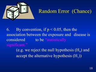
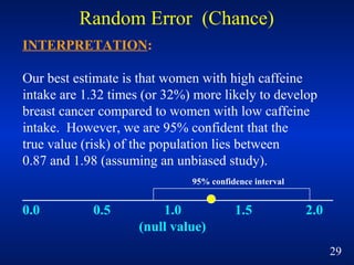
Introduction to Research Methods 
In the Internet Era 
Introduction to Biostatistics 
Inferential Statistics 
Hypothesis Testing 
Thomas Songer, PhD 
with acknowledgment to several slides provided by 
M Rahbar and Moataza Mahmoud Abdel Wahab
Key Lecture Concepts 
• Assess role of random error (chance) as an 
influence on the validity of the statistical 
association 
• Identify role of the p-value in statistical 
assessments 
• Identify role of the confidence interval in 
statistical assessments 
• Briefly introduce tests to undertake 
2
Research Process 
Research question 
Hypothesis 
Identify research design 
Data collection 
Presentation of data 
Data analysis 
Interpretation of data 
Polgar, Thomas 3
Interpreting Results 
When evaluating an association between 
disease and exposure, we need guidelines 
to help determine whether there is a 
true difference in the frequency of disease 
between the two exposure groups, or perhaps 
just random variation from the study sample. 
4
Random Error (Chance) 
1. Rarely can we study an entire population, so 
inference is attempted from a sample of 
the population 
2. There will always be random variation 
from sample to sample 
3. In general, smaller samples have less 
precision, reliability, and statistical power 
(more sampling variability) 
5
Hypothesis Testing 
• The process of deciding statistically 
whether the findings of an 
investigation reflect chance or real 
effects at a given level of probability. 
6
Elements of Testing hypothesis 
• Null Hypothesis 
• Alternative hypothesis 
• Identify level of significance 
• Test statistic 
• Identify p-value / confidence interval 
• Conclusion 
7
H0: There is no association between the 
exposure and disease of interest 
H1: There is an association between the 
exposure and disease of interest 
8 
Hypothesis Testing 
Note: With prudent skepticism, the null hypothesis 
is given the benefit of the doubt until the data 
convince us otherwise.
Hypothesis Testing 
• Because of statistical uncertainty regarding 
inferences about population parameters based 
upon sample data, we cannot prove or 
disprove either the null or alternate 
hypotheses as directly representing the 
population effect. 
• Thus, we make a decision based on 
probability and accept a probability of 
making an incorrect decision. 
Chernick 9
Associations 
• Two types of pitfalls can occur that 
affect the association between 
exposure and disease 
–Type 1 error: observing a difference 
when in truth there is none 
–Type 2 error: failing to observe a 
difference where there is one. 
10
Interpreting Epidemiologic Results 
Four possible outcomes of any epidemiologic study: 
YOUR 
DECISION 
H0 True 
(No assoc.) 
H1 True 
(Yes assoc.) 
Do not reject H0 
(not stat. sig.) 
Correct 
decision 
Type II 
(beta error) 
Reject H0 
(stat. sig.) 
Type I 
(alpha error) 
Correct 
decision 
11 
REALITY
Four possible outcomes of any epidemiologic study: 
YOUR 
DECISION 
H0 True 
(No assoc.) 
H1 True 
(Yes assoc.) 
Do not reject H0 
(not stat. sig.) 
Correct 
decision 
Failing to find a 
difference when 
one exists 
Reject H0 
(stat. sig.) 
Finding a 
difference when 
there is none 
Correct decision 
12 
REALITY
Type I and Type II errors 
"a is the probability of committing type I 
error. 
"b is the probability of committing type II 
error. 
13
“Conventional” Guidelines: 
• Set the fixed alpha level (Type I error) to 0.05 
This means, if the null hypothesis is true, the 
probability of incorrectly rejecting it is 5% or less. 
DECISION H0 True H1 True 
Do not reject H0 
(not stat. sig.) 
Reject H0 
(stat. sig.) 
Type I 
(alpha error) 
14 
Study Result
Empirical Rule 
For a Normal distribution approximately, 
a) 68% of the measurements fall within one 
standard deviation around the mean 
b) 95% of the measurements fall within two 
standard deviations around the mean 
c) 99.7% of the measurements fall within three 
standard deviations around the mean 
15
Normal Distribution 
34.13% 34.13% 
13.59% 
2.28% 
13.59% 
2.28% 
50% 50 % 
16 
• a usually set at 5%)
4. A test statistic to assess “statistical significance” 
is performed to assess the degree to which the 
data are compatible with the null hypothesis of no 
association 
5. Given a test statistic and an observed value, you 
can compute the probability of observing a value 
as extreme or more extreme than the observed 
value under the null hypothesis of no association. 
This probability is called the “p-value” 
17 
Random Error (Chance)
Random Error (Chance) 
6. By convention, if p < 0.05, then the 
association between the exposure and disease is 
considered to be “statistically 
significant.” 
(e.g. we reject the null hypothesis (H0) and 
accept the alternative hypothesis (H1)) 
18
Random Error (Chance) 
• p-value 
– the probability that an effect at least as 
extreme as that observed could have 
occurred by chance alone, given there is 
truly no relationship between exposure and 
disease (Ho) 
– the probability the observed results 
occurred by chance 
– that the sample estimates of association 
differ only because of sampling variability. 
Sever 19
What does p < 0.05 mean? 
Indirectly, it means that we suspect that the 
magnitude of effect observed (e.g. odds ratio) is 
not due to chance alone (in the absence of 
biased data collection or analysis) 
Directly, p=0.05 means that one test result out 
of twenty results would be expected to occur 
due to chance (random error) alone 
20 
Random Error (Chance)
Example: 
D+ D-E+ 
15 85 
E- 10 90 
IE+ = 15 / (15 + 85) = 0.15 
IE- = 10 / (10 + 90) = 0.10 
RR = IE+/IE- = 1.5, p = 0.30 
Although it appears that the incidence of disease may be 
higher in the exposed than in the non-exposed (RR=1.5), 
the p-value of 0.30 exceeds the fixed alpha level of 0.05. 
This means that the observed data are relatively 
compatible with the null hypothesis. Thus, we do not 
reject H0 in favor of H1 (alternative hypothesis). 
21
Random Error (Chance) 
Take Note: 
The p-value reflects both the magnitude of the 
difference between the study groups AND the 
sample size 
22 
• The size of the p-value does not 
indicate the importance of the results 
• Results may be statistically significant 
but be clinically unimportant 
• Results that are not statistically 
significant may still be important
23 
Sometimes we are more concerned with 
estimating the true difference than the 
probability that we are making the 
decision that the difference between 
samples is significant
Random Error (Chance) 
A related, but more informative, measure known 
as the confidence interval (CI) can also be 
calculated. 
CI = a range of values within which the true 
population value falls, with a certain degree of 
assurance (probability). 
24
Confidence Interval - Definition 
A range of values for a variable constructed 
so that this range has a specified 
probability of including the true value of 
the variable 
A measure of the study’s precision 
Lower limit Upper limit 
Sever 
Point estimate 
25
Statistical Measures of Chance 
• Confidence interval 
–95% C.I. means that true estimate of 
effect (mean, risk, rate) lies within 2 
standard errors of the population 
mean 95 times out of 100 
Sever 26
Interpreting Results 
Confidence Interval: Range of values for a point 
estimate that has a specified probability of 
including the true value of the parameter. 
Confidence Level: (1.0 – a), usually expressed 
as a percentage (e.g. 95%). 
Confidence Limits: The upper and lower end 
points of the confidence interval. 
27
Hypothetical Example of 95% Confidence Interval 
Exposure: Caffeine intake (high versus low) 
Outcome: Incidence of breast cancer 
Risk Ratio: 1.32 (point estimate) 
p-value: 0.14 (not statistically significant) 
95% C.I.: 0.87 - 1.98 
95% confidence interval 
_____________________________________________________ 
0.0 0.5 1.0 1.5 2.0 
28 
(null value)
INTERPRETATION: 
Our best estimate is that women with high caffeine 
intake are 1.32 times (or 32%) more likely to develop 
breast cancer compared to women with low caffeine 
intake. However, we are 95% confident that the 
true value (risk) of the population lies between 
0.87 and 1.98 (assuming an unbiased study). 
95% confidence interval 
_____________________________________________ 
0.0 0.5 1.0 1.5 2.0 
(null value) 
29 
Random Error (Chance)
If the 95% confidence interval does NOT include 
the null value of 1.0 (p < 0.05), then we declare a 
“statistically significant” association. 
If the 95% confidence interval includes the null 
value of 1.0, then the test result is “not statistically 
significant.” 
30 
Random Error (Chance) 
Interpretation:
Interpretation of C.I. For OR and RR: 
The C.I. provides an idea of the likely magnitude of 
the effect and the random variability of the point 
estimate. 
On the other hand, the p-value reveals nothing about 
the magnitude of the effect or the random variability 
of the point estimate. 
In general, smaller sample sizes have larger C.I.’s due 
to uncertainty (lack of precision) in the point estimate. 
31 
Interpreting Results
Selection of Tests of 
Significance 
32
Scale of Data 
1. Nominal: Data do not represent an amount or 
quantity (e.g., Marital Status, Sex) 
2. Ordinal: Data represent an ordered series of 
relationship (e.g., level of education) 
3. Interval: Data are measured on an interval scale 
having equal units but an arbitrary zero point. (e.g.: 
Temperature in Fahrenheit) 
4. Interval Ratio: Variable such as weight for which we 
can compare meaningfully one weight versus another 
(say, 100 Kg is twice 50 Kg) 33
Which Test to Use? 
Scale of Data 
Nominal Chi-square test 
Ordinal Mann-Whitney U test 
Interval (continuous) 
T-test 
- 2 groups 
Interval (continuous) 
- 3 or more groups 
ANOVA 
34
Tests for distributions 
• Common tests 
– For nominal data 
• with small counts – Fisher’s exact test >fisher.test() 
• with all counts >5 – Chi-squared test >chisq.test() 
• in case of dependent objects – McNemar test 
>mcnemar.test() 
– For continuous data 
• Kolmogorov-Smirnov test >ks.test() 
• Special tests 
– Normality tests 
• Shapiro-Wilks test >shapiro.test()
Tests for locations 
• Parametric tests 
– One-sample: t-test 
>t.test() 
– Two-sample, independent 
data: t-test >t.test() 
– Two-sample, dependent 
data: paired t-test 
>t.test(…, paired=TRUE) 
– Many samples, 
independent data: 
ANOVA >aov() 
– Many samples, dependent 
data: repeated 
measurements ANOVA 
>aov(…, error=…) 
• Nonparametric tests 
– One-sample: Wilcoxon sign 
test >wilcox.test() 
– Two-sample, independent 
data: Wilcoxon rank-sum 
test >wilcox.test() 
– Two-sample, dependent 
data: Wilcoxon signed-rank 
test >wilcox.test(…, 
paired=TRUE) 
– Many samples, independent 
data: Kruskal-Wallis test 
>kruskal.test() 
– Many samples, dependent 
data: Friedman test 
>friedman.test()
Tests for scales 
• Parametric tests 
– Two-sample: Fisher’s 
test >f.test() 
– Many samples: 
Bartlett’s test 
>bartlett.test() 
• Nonparametric tests 
– Two-sample: Ansari- 
Bradley test 
>ansari.test() 
– Many samples: Fligner- 
Killeen test 
>fligner.test()

Lecture2 hypothesis testing

  • 1.
    Introduction to ResearchMethods In the Internet Era Introduction to Biostatistics Inferential Statistics Hypothesis Testing Thomas Songer, PhD with acknowledgment to several slides provided by M Rahbar and Moataza Mahmoud Abdel Wahab
  • 2.
    Key Lecture Concepts • Assess role of random error (chance) as an influence on the validity of the statistical association • Identify role of the p-value in statistical assessments • Identify role of the confidence interval in statistical assessments • Briefly introduce tests to undertake 2
  • 3.
    Research Process Researchquestion Hypothesis Identify research design Data collection Presentation of data Data analysis Interpretation of data Polgar, Thomas 3
  • 4.
    Interpreting Results Whenevaluating an association between disease and exposure, we need guidelines to help determine whether there is a true difference in the frequency of disease between the two exposure groups, or perhaps just random variation from the study sample. 4
  • 5.
    Random Error (Chance) 1. Rarely can we study an entire population, so inference is attempted from a sample of the population 2. There will always be random variation from sample to sample 3. In general, smaller samples have less precision, reliability, and statistical power (more sampling variability) 5
  • 6.
    Hypothesis Testing •The process of deciding statistically whether the findings of an investigation reflect chance or real effects at a given level of probability. 6
  • 7.
    Elements of Testinghypothesis • Null Hypothesis • Alternative hypothesis • Identify level of significance • Test statistic • Identify p-value / confidence interval • Conclusion 7
  • 8.
    H0: There isno association between the exposure and disease of interest H1: There is an association between the exposure and disease of interest 8 Hypothesis Testing Note: With prudent skepticism, the null hypothesis is given the benefit of the doubt until the data convince us otherwise.
  • 9.
    Hypothesis Testing •Because of statistical uncertainty regarding inferences about population parameters based upon sample data, we cannot prove or disprove either the null or alternate hypotheses as directly representing the population effect. • Thus, we make a decision based on probability and accept a probability of making an incorrect decision. Chernick 9
  • 10.
    Associations • Twotypes of pitfalls can occur that affect the association between exposure and disease –Type 1 error: observing a difference when in truth there is none –Type 2 error: failing to observe a difference where there is one. 10
  • 11.
    Interpreting Epidemiologic Results Four possible outcomes of any epidemiologic study: YOUR DECISION H0 True (No assoc.) H1 True (Yes assoc.) Do not reject H0 (not stat. sig.) Correct decision Type II (beta error) Reject H0 (stat. sig.) Type I (alpha error) Correct decision 11 REALITY
  • 12.
    Four possible outcomesof any epidemiologic study: YOUR DECISION H0 True (No assoc.) H1 True (Yes assoc.) Do not reject H0 (not stat. sig.) Correct decision Failing to find a difference when one exists Reject H0 (stat. sig.) Finding a difference when there is none Correct decision 12 REALITY
  • 13.
    Type I andType II errors "a is the probability of committing type I error. "b is the probability of committing type II error. 13
  • 14.
    “Conventional” Guidelines: •Set the fixed alpha level (Type I error) to 0.05 This means, if the null hypothesis is true, the probability of incorrectly rejecting it is 5% or less. DECISION H0 True H1 True Do not reject H0 (not stat. sig.) Reject H0 (stat. sig.) Type I (alpha error) 14 Study Result
  • 15.
    Empirical Rule Fora Normal distribution approximately, a) 68% of the measurements fall within one standard deviation around the mean b) 95% of the measurements fall within two standard deviations around the mean c) 99.7% of the measurements fall within three standard deviations around the mean 15
  • 16.
    Normal Distribution 34.13%34.13% 13.59% 2.28% 13.59% 2.28% 50% 50 % 16 • a usually set at 5%)
  • 17.
    4. A teststatistic to assess “statistical significance” is performed to assess the degree to which the data are compatible with the null hypothesis of no association 5. Given a test statistic and an observed value, you can compute the probability of observing a value as extreme or more extreme than the observed value under the null hypothesis of no association. This probability is called the “p-value” 17 Random Error (Chance)
  • 18.
    Random Error (Chance) 6. By convention, if p < 0.05, then the association between the exposure and disease is considered to be “statistically significant.” (e.g. we reject the null hypothesis (H0) and accept the alternative hypothesis (H1)) 18
  • 19.
    Random Error (Chance) • p-value – the probability that an effect at least as extreme as that observed could have occurred by chance alone, given there is truly no relationship between exposure and disease (Ho) – the probability the observed results occurred by chance – that the sample estimates of association differ only because of sampling variability. Sever 19
  • 20.
    What does p< 0.05 mean? Indirectly, it means that we suspect that the magnitude of effect observed (e.g. odds ratio) is not due to chance alone (in the absence of biased data collection or analysis) Directly, p=0.05 means that one test result out of twenty results would be expected to occur due to chance (random error) alone 20 Random Error (Chance)
  • 21.
    Example: D+ D-E+ 15 85 E- 10 90 IE+ = 15 / (15 + 85) = 0.15 IE- = 10 / (10 + 90) = 0.10 RR = IE+/IE- = 1.5, p = 0.30 Although it appears that the incidence of disease may be higher in the exposed than in the non-exposed (RR=1.5), the p-value of 0.30 exceeds the fixed alpha level of 0.05. This means that the observed data are relatively compatible with the null hypothesis. Thus, we do not reject H0 in favor of H1 (alternative hypothesis). 21
  • 22.
    Random Error (Chance) Take Note: The p-value reflects both the magnitude of the difference between the study groups AND the sample size 22 • The size of the p-value does not indicate the importance of the results • Results may be statistically significant but be clinically unimportant • Results that are not statistically significant may still be important
  • 23.
    23 Sometimes weare more concerned with estimating the true difference than the probability that we are making the decision that the difference between samples is significant
  • 24.
    Random Error (Chance) A related, but more informative, measure known as the confidence interval (CI) can also be calculated. CI = a range of values within which the true population value falls, with a certain degree of assurance (probability). 24
  • 25.
    Confidence Interval -Definition A range of values for a variable constructed so that this range has a specified probability of including the true value of the variable A measure of the study’s precision Lower limit Upper limit Sever Point estimate 25
  • 26.
    Statistical Measures ofChance • Confidence interval –95% C.I. means that true estimate of effect (mean, risk, rate) lies within 2 standard errors of the population mean 95 times out of 100 Sever 26
  • 27.
    Interpreting Results ConfidenceInterval: Range of values for a point estimate that has a specified probability of including the true value of the parameter. Confidence Level: (1.0 – a), usually expressed as a percentage (e.g. 95%). Confidence Limits: The upper and lower end points of the confidence interval. 27
  • 28.
    Hypothetical Example of95% Confidence Interval Exposure: Caffeine intake (high versus low) Outcome: Incidence of breast cancer Risk Ratio: 1.32 (point estimate) p-value: 0.14 (not statistically significant) 95% C.I.: 0.87 - 1.98 95% confidence interval _____________________________________________________ 0.0 0.5 1.0 1.5 2.0 28 (null value)
  • 29.
    INTERPRETATION: Our bestestimate is that women with high caffeine intake are 1.32 times (or 32%) more likely to develop breast cancer compared to women with low caffeine intake. However, we are 95% confident that the true value (risk) of the population lies between 0.87 and 1.98 (assuming an unbiased study). 95% confidence interval _____________________________________________ 0.0 0.5 1.0 1.5 2.0 (null value) 29 Random Error (Chance)
  • 30.
    If the 95%confidence interval does NOT include the null value of 1.0 (p < 0.05), then we declare a “statistically significant” association. If the 95% confidence interval includes the null value of 1.0, then the test result is “not statistically significant.” 30 Random Error (Chance) Interpretation:
  • 31.
    Interpretation of C.I.For OR and RR: The C.I. provides an idea of the likely magnitude of the effect and the random variability of the point estimate. On the other hand, the p-value reveals nothing about the magnitude of the effect or the random variability of the point estimate. In general, smaller sample sizes have larger C.I.’s due to uncertainty (lack of precision) in the point estimate. 31 Interpreting Results
  • 32.
    Selection of Testsof Significance 32
  • 33.
    Scale of Data 1. Nominal: Data do not represent an amount or quantity (e.g., Marital Status, Sex) 2. Ordinal: Data represent an ordered series of relationship (e.g., level of education) 3. Interval: Data are measured on an interval scale having equal units but an arbitrary zero point. (e.g.: Temperature in Fahrenheit) 4. Interval Ratio: Variable such as weight for which we can compare meaningfully one weight versus another (say, 100 Kg is twice 50 Kg) 33
  • 34.
    Which Test toUse? Scale of Data Nominal Chi-square test Ordinal Mann-Whitney U test Interval (continuous) T-test - 2 groups Interval (continuous) - 3 or more groups ANOVA 34
  • 37.
    Tests for distributions • Common tests – For nominal data • with small counts – Fisher’s exact test >fisher.test() • with all counts >5 – Chi-squared test >chisq.test() • in case of dependent objects – McNemar test >mcnemar.test() – For continuous data • Kolmogorov-Smirnov test >ks.test() • Special tests – Normality tests • Shapiro-Wilks test >shapiro.test()
  • 38.
    Tests for locations • Parametric tests – One-sample: t-test >t.test() – Two-sample, independent data: t-test >t.test() – Two-sample, dependent data: paired t-test >t.test(…, paired=TRUE) – Many samples, independent data: ANOVA >aov() – Many samples, dependent data: repeated measurements ANOVA >aov(…, error=…) • Nonparametric tests – One-sample: Wilcoxon sign test >wilcox.test() – Two-sample, independent data: Wilcoxon rank-sum test >wilcox.test() – Two-sample, dependent data: Wilcoxon signed-rank test >wilcox.test(…, paired=TRUE) – Many samples, independent data: Kruskal-Wallis test >kruskal.test() – Many samples, dependent data: Friedman test >friedman.test()
  • 39.
    Tests for scales • Parametric tests – Two-sample: Fisher’s test >f.test() – Many samples: Bartlett’s test >bartlett.test() • Nonparametric tests – Two-sample: Ansari- Bradley test >ansari.test() – Many samples: Fligner- Killeen test >fligner.test()

Editor's Notes

  • #2 All lectures from Workshop - http://www.pitt.edu/~super1/CentralAsia/workshop.htm This project is made possible by the support of the American people through the United States Agency for International Development (USAID). The contents are the sole responsibility of the University of Pittsburgh and do not necessarily reflect the views of USAID or the United States  Government.
  • #3 The fundamental concepts of this lecture are outlined here.