Estimation and hypothesis techniques

1. Estimation and Hypothesis Testing

2. Objectives
 After complete this session you will be able to do
 Parameter estimations
◼ Point estimate
◼ Confidence interval
 Hypothesis testing
◼ Z-test
◼ T-test
 Testing associations
◼ Chi-Square test
2

3. Introduction # 1
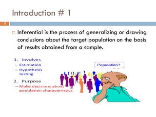
 Inferential is the process of generalizing or drawing
conclusions about the target population on the basis
of results obtained from a sample.
3

4. Introduction #2
 Before beginning statistical analyses
 it is essential to examine the distribution of the variable for
skewness (tails),
 kurtosis (peaked or flat distribution), spread (range of the
values) and
 outliers (data values separated from the rest of the data).
 Information about each of these characteristics
determines to choose the statistical analyses and can
be accurately explained and interpreted.
4

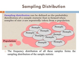
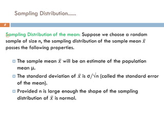
5. Sampling Distribution
 The frequency distribution of all these samples forms the
sampling distribution of the sample statistic
5

6. Sampling distribution .......
6
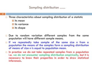
 Three characteristics about sampling distribution of a statistic
 its mean
 its variance
 its shape
 Due to random variation different samples from the same
population will have different sample means.
 If we repeatedly take sample of the same size n from a
population the means of the samples form a sampling distribution
of means of size n is equal to population mean.
 In practice we do not take repeated samples from a population
i.e. we do not encounter sampling distribution empirically, but it is
necessary to know their properties in order to draw statistical
inferences.

7. The Central Limit Theorem
7
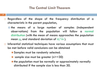
 Regardless of the shape of the frequency distribution of a
characteristic in the parent population,
 the means of a large number of samples (independent
observations) from the population will follow a normal
distribution (with the mean of means approaches the population
mean μ, and standard deviation of σ/√n ).
 Inferential statistical techniques have various assumptions that must
be met before valid conclusions can be obtained
◼ Samples must be randomly selected.
◼ sample size must be greater (n>=30)
◼ the population must be normally or approximately normally
distributed if the sample size is less than 30.

8. Sampling Distribution......
8


9. Sampling Distribution ..........
9


10. Standard deviation and Standard error
Standard deviation is a measure of variability between
individual observations (descriptive index relevant to
mean)
Standard error refers to the variability of summary
statistics (e.g. the variability of the sample mean or a
sample proportion)
Standard error is a measure of uncertainty in a sample
statistics i.e. precision of the estimate of the estimator

11. Parameter Estimations
11
 In parameter estimation, we generally assume that the
underlying (unknown) distribution of the variable of interest is
adequately described by one or more (unknown) parameters,
referred as population parameters.
 As it is usually not possible to make measurements on every
individual in a population, parameters cannot usually be
determined exactly.
 Instead we estimate parameters by calculating the
corresponding characteristics from a random sample estimates .
 the process of estimating the value of a parameter from
information obtained from a sample.

12. Estimation
Estimation is a procedure in which we use the information
included in a sample to get inferences about the true
parameter of interest.
 An estimator is a sample statistic that used to estimate the
population parameter while an estimate is the possible values
that a given estimator can assume.

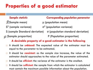
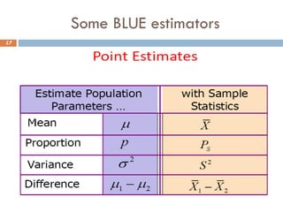
13. Properties of a good estimator
Sample statistic Corresponding population parameter
(Sample mean) μ (population mean)
S2 (sample variance) σ2 (population variance)
S (sample Standard deviation) σ (population standard deviation)
(Sample proportion) P (Population proportion)
A desirable property of a good estimator is the following
 It should be unbiased: The expected value of the estimator must be
equal to the parameter to be estimated.
 It should be consistent: as the sample size increase, the value of the
estimator should approaches to the value of the parameter estimated.
 It should be efficient: the variance of the estimator is the smallest.
 It should be sufficient: the sample from which the estimator is calculated
must contain the maximum possible information about the population.

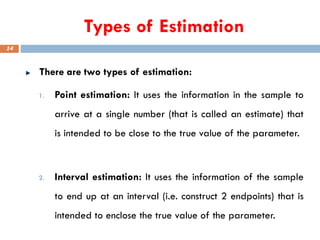
14. Types of Estimation
There are two types of estimation:
1. Point estimation: It uses the information in the sample to
arrive at a single number (that is called an estimate) that
is intended to be close to the true value of the parameter.
2. Interval estimation: It uses the information of the sample
to end up at an interval (i.e. construct 2 endpoints) that is
intended to enclose the true value of the parameter.
14

15. Point Estimation
15

n
=
p
x


16. Example


17. Some BLUE estimators
17

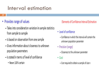
18. Interval Estimation
18
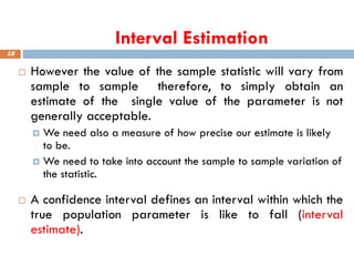
 However the value of the sample statistic will vary from
sample to sample therefore, to simply obtain an
estimate of the single value of the parameter is not
generally acceptable.
 We need also a measure of how precise our estimate is likely
to be.
 We need to take into account the sample to sample variation of
the statistic.
 A confidence interval defines an interval within which the
true population parameter is like to fall (interval
estimate).

19. Confidence Intervals…
19
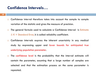
 Confidence interval therefore takes into account the sample to sample
variation of the statistic and gives the measure of precision.
 The general formula used to calculate a Confidence interval is Estimate
± K × Standard Error, k is called reliability coefficient.
 Confidence intervals express the inherent uncertainty in any medical
study by expressing upper and lower bounds for anticipated true
underlying population parameter.
 The confidence level is the probability that the interval estimate will
contain the parameter, assuming that a large number of samples are
selected and that the estimation process on the same parameter is
repeated.

20. Confidence intervals…
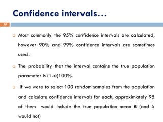
❑ Most commonly the 95% confidence intervals are calculated,
however 90% and 99% confidence intervals are sometimes
used.
❑ The probability that the interval contains the true population
parameter is (1-α)100%.
❑ If we were to select 100 random samples from the population
and calculate confidence intervals for each, approximately 95
of them would include the true population mean B (and 5
would not)
20

21. Confidence interval ……
21
]
/
)
1
(
.
,
/
)
1
(
.
[
]
.
,
.
[
2
2
2
2
n
p
p
z
p
n
p
p
z
p
n
z
x
n
z
x
−
+
−
−

+
−









A (1-α) 100% confidence interval for unknown population
mean and population proportion is given as follows;

22. Interval estimation
22

23. 23

24. 24

25. 25

26. Confidence intervals…
26
 The 95% confidence interval is calculated in such a way that, under the
conditions assumed for underlying distribution, the interval will contain true
population parameter 95% of the time.
 Loosely speaking, you might interpret a 95% confidence interval as one which
you are 95% confident contains the true parameter.
 90% CI is narrower than 95% CI since we are only 90% certain that the interval
includes the population parameter.
 On the other hand 99% CI will be wider than 95% CI; the extra width meaning
that we can be more certain that the interval will contain the population
parameter. But to obtain a higher confidence from the same sample, we must be
willing to accept a larger margin of error (a wider interval).

27. Confidence intervals…
27
 For a given confidence level (i.e. 90%, 95%, 99%) the
width of the confidence interval depends on the
standard error of the estimate which in turn depends on
the
 1. Sample size:-The larger the sample size, the narrower the
confidence interval (this is to mean the sample statistic will
approach the population parameter) and the more precise our
estimate. Lack of precision means that in repeated sampling
the values of the sample statistic are spread out or scattered.
The result of sampling is not repeatable.

28. Confidence intervals…
28


29. Confidence interval for a single mean
CI =
Most commonly, we used to compute 95% confidence
interval, however, it is possible to compute 90% and 99%
confidence interval estimation.

30. Area between 0 and z
0.00 0.01 0.02 0.03 0.04 0.05 0.06 0.07 0.08 0.09
0.0 0.0000 0.0040 0.0080 0.0120 0.0160 0.0199 0.0239 0.0279 0.0319 0.0359
0.1 0.0398 0.0438 0.0478 0.0517 0.0557 0.0596 0.0636 0.0675 0.0714 0.0753
0.2 0.0793 0.0832 0.0871 0.0910 0.0948 0.0987 0.1026 0.1064 0.1103 0.1141
0.3 0.1179 0.1217 0.1255 0.1293 0.1331 0.1368 0.1406 0.1443 0.1480 0.1517
0.4 0.1554 0.1591 0.1628 0.1664 0.1700 0.1736 0.1772 0.1808 0.1844 0.1879
0.5 0.1915 0.1950 0.1985 0.2019 0.2054 0.2088 0.2123 0.2157 0.2190 0.2224
0.6 0.2257 0.2291 0.2324 0.2357 0.2389 0.2422 0.2454 0.2486 0.2517 0.2549
0.7 0.2580 0.2611 0.2642 0.2673 0.2704 0.2734 0.2764 0.2794 0.2823 0.2852
0.8 0.2881 0.2910 0.2939 0.2967 0.2995 0.3023 0.3051 0.3078 0.3106 0.3133
0.9 0.3159 0.3186 0.3212 0.3238 0.3264 0.3289 0.3315 0.3340 0.3365 0.3389
1.0 0.3413 0.3438 0.3461 0.3485 0.3508 0.3531 0.3554 0.3577 0.3599 0.3621
1.1 0.3643 0.3665 0.3686 0.3708 0.3729 0.3749 0.3770 0.3790 0.3810 0.3830
1.2 0.3849 0.3869 0.3888 0.3907 0.3925 0.3944 0.3962 0.3980 0.3997 0.4015
1.3 0.4032 0.4049 0.4066 0.4082 0.4099 0.4115 0.4131 0.4147 0.4162 0.4177
1.4 0.4192 0.4207 0.4222 0.4236 0.4251 0.4265 0.4279 0.4292 0.4306 0.4319
1.5 0.4332 0.4345 0.4357 0.4370 0.4382 0.4394 0.4406 0.4418 0.4429 0.4441
1.6 0.4452 0.4463 0.4474 0.4484 0.4495 0.4505 0.4515 0.4525 0.4535 0.4545
1.7 0.4554 0.4564 0.4573 0.4582 0.4591 0.4599 0.4608 0.4616 0.4625 0.4633
1.8 0.4641 0.4649 0.4656 0.4664 0.4671 0.4678 0.4686 0.4693 0.4699 0.4706
1.9 0.4713 0.4719 0.4726 0.4732 0.4738 0.4744 0.4750 0.4756 0.4761 0.4767
2.0 0.4772 0.4778 0.4783 0.4788 0.4793 0.4798 0.4803 0.4808 0.4812 0.4817
2.1 0.4821 0.4826 0.4830 0.4834 0.4838 0.4842 0.4846 0.4850 0.4854 0.4857
2.2 0.4861 0.4864 0.4868 0.4871 0.4875 0.4878 0.4881 0.4884 0.4887 0.4890
2.3 0.4893 0.4896 0.4898 0.4901 0.4904 0.4906 0.4909 0.4911 0.4913 0.4916
30
Table 1: Normal distribution

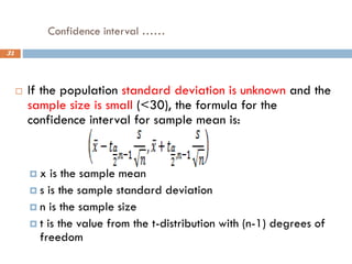
31. Confidence interval ……
31
 If the population standard deviation is unknown and the
sample size is small (<30), the formula for the
confidence interval for sample mean is:
 x is the sample mean
 s is the sample standard deviation
 n is the sample size
 t is the value from the t-distribution with (n-1) degrees of
freedom

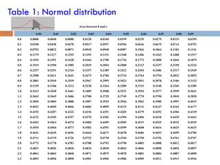
32. df t0.100 t0.050 t0.025 t0.010 t0.005
--- ----- ----- ------ ------ ------
1 3.078 6.314 12.706 31.821 63.657
2 1.886 2.920 4.303 6.965 9.925
3 1.638 2.353 3.182 4.541 5.841
4 1.533 2.132 2.776 3.747 4.604
5 1.476 2.015 2.571 3.365 4.032
6 1.440 1.943 2.447 3.143 3.707
7 1.415 1.895 2.365 2.998 3.499
8 1.397 1.860 2.306 2.896 3.355
9 1.383 1.833 2.262 2.821 3.250
10 1.372 1.812 2.228 2.764 3.169
11 1.363 1.796 2.201 2.718 3.106
12 1.356 1.782 2.179 2.681 3.055
13 1.350 1.771 2.160 2.650 3.012
14 1.345 1.761 2.145 2.624 2.977
15 1.341 1.753 2.131 2.602 2.947
16 1.337 1.746 2.120 2.583 2.921
17 1.333 1.740 2.110 2.567 2.898
18 1.330 1.734 2.101 2.552 2.878
19 1.328 1.729 2.093 2.539 2.861
20 1.325 1.725 2.086 2.528 2.845
21 1.323 1.721 2.080 2.518 2.831
22 1.321 1.717 2.074 2.508 2.819
23 1.319 1.714 2.069 2.500 2.807
24 1.318 1.711 2.064 2.492 2.797
25 1.316 1.708 2.060 2.485 2.787
26 1.315 1.706 2.056 2.479 2.779
27 1.314 1.703 2.052 2.473 2.771
28 1.313 1.701 2.048 2.467 2.763
29 1.311 1.699 2.045 2.462 2.756
30 1.310 1.697 2.042 2.457 2.750
40 1.303 1.684 2.021 2.423 2.704
60 1.296 1.671 2.000 2.390 2.660
120 1.289 1.658 1.980 2.358 2.617
1.282 1.645 1.960 2.326 2.576

0
0 .4
0 .3
0 .2
0 .1
0 .0
t
f(t)
t D istrib utio n: d f=10
Area = 0.10
}
Area = 0.10
}
Area = 0.025
}
Area = 0.025
}
1.372
-1.372
2.228
-2.228
Whenever  is not known (and the population is
assumed normal), the correct distribution to use is
the t distribution with n-1 degrees of freedom.
Note, however, that for large degrees of freedom,
the t distribution is approximated well by the Z
distribution.
The t Distribution
32

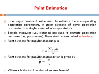
33. Point and Interval Estimation of the Population Proportion (p)
We will now consider the method for estimating the binomial
proportion p of successes, that is, the proportion of elements in a
population that have a certain characteristic.
A logical candidate for a point estimate of the population
proportion p is the sample proportion , where x is the number
of observations in a sample of size n that have the characteristic
of interest. As we have seen in sampling distribution of proportions,
the sample proportion is the best point estimate of the population
proportion.
n
x
p =
ˆ

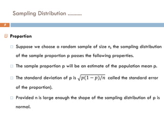
34. Proportion…
34
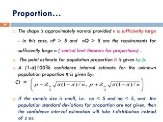
 The shape is approximately normal provided n is sufficiently large
- in this case, nP > 5 and nQ > 5 are the requirements for
sufficiently large n ( central limit theorem for proportions) .
❑ The point estimate for population proportion π is given by þ.
❑ A (1-α)100% confidence interval estimate for the unknown
population proportion π is given by:
CI =
❑ If the sample size is small, i.e. np < 5 and nq < 5, and the
population standard deviations for proportion are not given, then
the confidence interval estimation will take t-distribution instead
of z as:








−
+
−
− n
Z
p
n
Z
p /
)
1
(
,
/
)
1
(
2
2



 


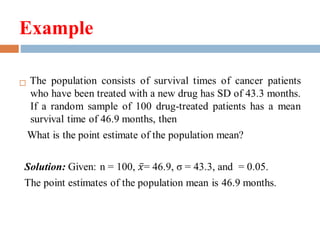
35. Example 1:
35
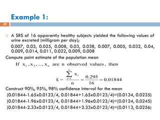
 A SRS of 16 apparently healthy subjects yielded the following values of
urine excreted (milligram per day);
0.007, 0.03, 0.025, 0.008, 0.03, 0.038, 0.007, 0.005, 0.032, 0.04,
0.009, 0.014, 0.011, 0.022, 0.009, 0.008
Compute point estimate of the population mean
Construct 90%, 95%, 98% confidence interval for the mean
(0.01844-1.65x0.0123/4, 0.01844+1.65x0.0123/4)=(0.0134, 0.0235)
(0.01844-1.96x0.0123/4, 0.01844+1.96x0.0123/4)=(0.0124, 0.0245)
(0.01844-2.33x0.0123/4, 0.01844+2.33x0.0123/4)=(0.0113, 0.0256)
01844
.
0
16
295
.
0
n
x
=
x
then
,
values
observed
n
are
x
...,
,
x
,
x
If
n
1
=
i
i
n
2
1
=
=


36. Example 2
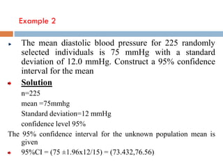
The mean diastolic blood pressure for 225 randomly
selected individuals is 75 mmHg with a standard
deviation of 12.0 mmHg. Construct a 95% confidence
interval for the mean
Solution
n=225
mean =75mmhg
Standard deviation=12 mmHg
confidence level 95%
The 95% confidence interval for the unknown population mean is
given
95%CI = (75 ±1.96x12/15) = (73.432,76.56)

37. Example 3:
38
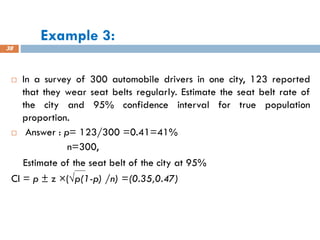
 In a survey of 300 automobile drivers in one city, 123 reported
that they wear seat belts regularly. Estimate the seat belt rate of
the city and 95% confidence interval for true population
proportion.
 Answer : p= 123/300 =0.41=41%
n=300,
Estimate of the seat belt of the city at 95%
CI = p ± z ×(√p(1-p) /n) =(0.35,0.47)

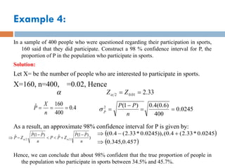
38. Example 4:
In a sample of 400 people who were questioned regarding their participation in sports,
160 said that they did participate. Construct a 98 % confidence interval for P, the
proportion of P in the population who participate in sports.
Solution:
Let X= be the number of people who are interested to participate in sports.
X=160, n=400, =0.02, Hence
As a result, an approximate 98% confidence interval for P is given by:
Hence, we can conclude that about 98% confident that the true proportion of people in
the population who participate in sports between 34.5% and 45.7%.
33
.
2
01
.
0
2 =
= Z
Z

4
.
0
400
160
ˆ =
=
=
n
X
P 0245
.
0
400
)
6
.
0
(
4
.
0
)
1
(
2
ˆ =
=
−
=
n
P
P
P

)
)
ˆ
1
(
ˆ
ˆ
)
ˆ
1
(
ˆ
ˆ
2
2
n
P
P
Z
P
P
n
P
P
Z
P
−
+


−
−
 

( )
( )
457
.
0
,
345
.
0
0245
.
0
*
33
.
2
(
4
.
0
(
)),
0245
.
0
*
33
.
2
(
4
.
0
(

+
−


39. HYPOTHESIS TESTING
40
Introduction
 Researchers are interested in answering many types of
questions. For example, A physician might want to know
whether a new medication will lower a person’s blood
pressure.
 These types of questions can be addressed through
statistical hypothesis testing, which is a decision-making
process for evaluating claims about a population.

40. Hypothesis Testing
41
 The formal process of hypothesis testing provides us with a means
of answering research questions.
 Hypothesis is a testable statement that describes the nature of
the proposed relationship between two or more variables of
interest.
 In hypothesis testing, the researcher must defined the population
under study, state the particular hypotheses that will be
investigated, give the significance level, select a sample from the
population, collect the data, perform the calculations required for
the statistical test, and reach a conclusion.

41. Idea of hypothesis testing
42

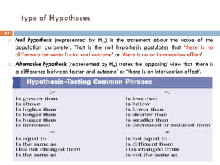
42. type of Hypotheses
43
 Null hypothesis (represented by HO) is the statement about the value of the
population parameter. That is the null hypothesis postulates that ‘there is no
difference between factor and outcome’ or ‘there is no an intervention effect’.
 Alternative hypothesis (represented by HA) states the ‘opposing’ view that ‘there is
a difference between factor and outcome’ or ‘there is an intervention effect’.

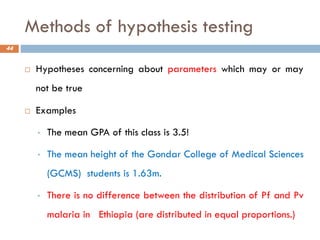
43. Methods of hypothesis testing
 Hypotheses concerning about parameters which may or may
not be true
 Examples
• The mean GPA of this class is 3.5!
• The mean height of the Gondar College of Medical Sciences
(GCMS) students is 1.63m.
• There is no difference between the distribution of Pf and Pv
malaria in Ethiopia (are distributed in equal proportions.)
44

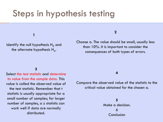
44. Steps in hypothesis testing
45
1
Identify the null hypothesis H0 and
the alternate hypothesis HA.
3
Select the test statistic and determine
its value from the sample data. This
value is called the observed value of
the test statistic. Remember that t
statistic is usually appropriate for a
small number of samples; for larger
number of samples, a z statistic can
work well if data are normally
distributed.
4
Compare the observed value of the statistic to the
critical value obtained for the chosen a.
5
Make a decision.
6
Conclusion
2
Choose a. The value should be small, usually less
than 10%. It is important to consider the
consequences of both types of errors.

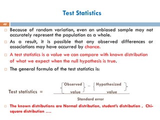
45. Test Statistics
46
 Because of random variation, even an unbiased sample may not
accurately represent the population as a whole.
 As a result, it is possible that any observed differences or
associations may have occurred by chance.
 A test statistics is a value we can compare with known distribution
of what we expect when the null hypothesis is true.
 The general formula of the test statistics is:
Observed _ Hypothesized
Test statistics = value value .
Standard error
 The known distributions are Normal distribution, student’s distribution , Chi-
square distribution ….

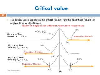
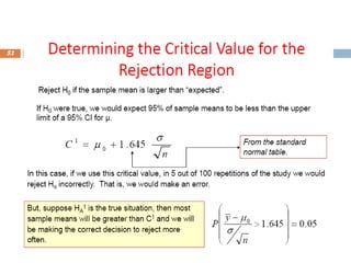
46. Critical value
 The critical value separates the critical region from the noncritical region for
a given level of significance
47

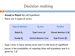
47. Decision making
48
 Accept or Reject the null hypothesis
 There are 2 types of errors
 Type I error is more serious error and it is the level of significant
 power is the probability of rejecting false null hypothesis and it is
given by 1-β
Type of decision H0 true H0 false
Reject H0 Type I error (a) Correct decision (1-β)
Accept H0 Correct decision (1-a) Type II error (β)

48. 49

49. 50

50. 51

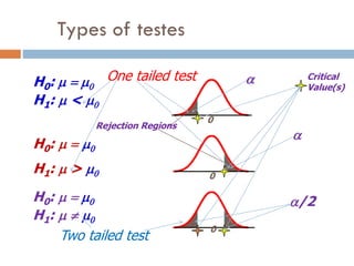
51. H0: m = m0
H1: m < m0
0
0
0
H0: m = m0
H1: m > m0
H0: m = m0
H1: m  m0


/2
Critical
Value(s)
Rejection Regions
One tailed test
Two tailed test
Types of testes

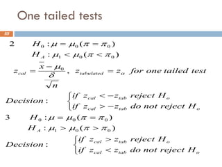
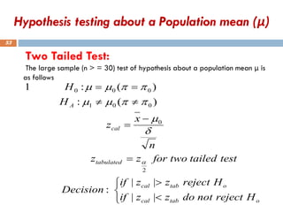
52. Two Tailed Test:
The large sample (n > = 30) test of hypothesis about a population mean μ is
as follows
53





=
−
=


=
=
o
tab
cal
o
tab
cal
tabulated
cal
A
H
reject
not
do
z
z
if
H
reject
z
z
if
Decision
test
tailed
two
for
z
z
n
x
z
H
H
|
|
|
|
:
)
(
:
)
(
:
1
2
0
0
0
1
0
0
0


m


m
m


m
m
Hypothesis testing about a Population mean (μ)

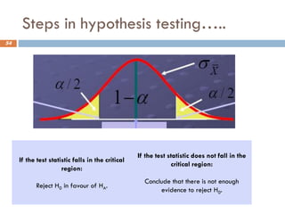
53. Steps in hypothesis testing…..
54
If the test statistic falls in the critical
region:
Reject H0 in favour of HA.
If the test statistic does not fall in the
critical region:
Conclude that there is not enough
evidence to reject H0.

54. One tailed tests
55







=
=



−

−

=
−
=


=
=
o
tab
cal
o
tab
cal
A
o
tab
cal
o
tab
cal
tabulated
cal
A
H
reject
not
do
z
z
if
H
reject
z
z
if
Decision
H
H
H
reject
not
do
z
z
if
H
reject
z
z
if
Decision
test
tailed
one
for
z
z
n
x
z
H
H
:
)
(
:
)
(
:
3
:
,
)
(
:
)
(
:
2
0
0
1
0
0
0
0
0
0
1
0
0
0


m
m


m
m

m


m
m


m
m


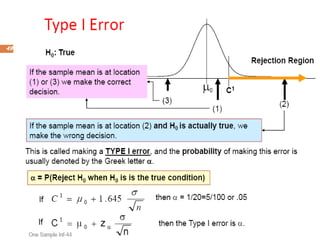
55. The P- Value
56
 In most applications, the outcome of performing a hypothesis test is
to produce a p-value.
 P-value is the probability that the observed difference is due to
chance.
 A large p-value implies that the probability of the value observed,
occurring just by chance is low, when the null hypothesis is true.
 That is, a small p-value suggests that there might be sufficient
evidence for rejecting the null hypothesis.
 The p value is defined as the probability of observing the
computed significance test value or a larger one, if the H0
hypothesis is true. For example, P[ Z >=Zcal/H0 true].

56. P-value……
 A p-value is the probability of getting the
observed difference, or one more extreme, in the
sample purely by chance from a population where
the true difference is zero.
 If the p-value is greater than 0.05 then, by
convention, we conclude that the observed difference
could have occurred by chance and there is no
statistically significant evidence (at the 5% level) for
a difference between the groups in the population.
57

57. How to calculate P-value
o Use statistical software like SPSS, SAS……..
o Hand calculations
—obtained the test statistics (Z Calculated or t-
calculated)
—find the probability of test statistics from standard
normal table
—subtract the probability from 0.5
—the result is P-value
Note if the test two tailed multiply 2 the result.

58. P-value and confidence interval
 Confidence intervals and p-values are based upon the same
theory and mathematics and will lead to the same conclusion
about whether a population difference exists.
 Confidence intervals are referable because they give
information about the size of any difference in the population,
and they also (very usefully) indicate the amount of uncertainty
remaining about the size of the difference.
 When the null hypothesis is rejected in a hypothesis-testing
situation, the confidence interval for the mean using the same
level of significance will not contain the hypothesized mean.
59

59. The P- Value …..
60
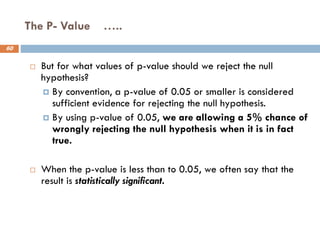
 But for what values of p-value should we reject the null
hypothesis?
 By convention, a p-value of 0.05 or smaller is considered
sufficient evidence for rejecting the null hypothesis.
 By using p-value of 0.05, we are allowing a 5% chance of
wrongly rejecting the null hypothesis when it is in fact
true.
 When the p-value is less than to 0.05, we often say that the
result is statistically significant.

60. Hypothesis testing for single population mean
61
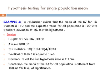
EXAMPLE 5: A researcher claims that the mean of the IQ for 16
students is 110 and the expected value for all population is 100 with
standard deviation of 10. Test the hypothesis .
 Solution
1. Ho:µ=100 VS HA:µ≠100
2. Assume α=0.05
3. Test statistics: z=(110-100)4/10=4
4. z-critical at 0.025 is equal to 1.96.
5. Decision: reject the null hypothesis since 4 ≥ 1.96
6. Conclusion: the mean of the IQ for all population is different from
100 at 5% level of significance.

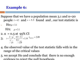
61. Example 6:
Suppose that we have a population mean 3.1 and n=20
people and found and , our test statistic is
1. Ho:
HA:
2. α = 0.5 at 95% CI
3.
4. the observed value of the test statistic falls with in the
range of the critical values
5. we accept Ho and conclude that there is no enough
62
14
.
1
20
5
.
5
1
.
3
5
.
4
=
−
=
−
=
n
s
x
t
m 09
.
2
19
,
05
.
0 =
t
5
.
4
=
x 5
.
5
=
s
1
.
3

m
1
.
3
=
m

62. Cont….
63
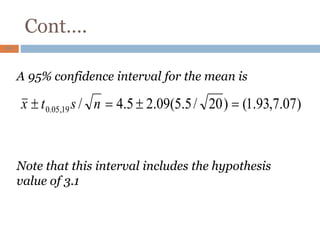
A 95% confidence interval for the mean is
Note that this interval includes the hypothesis
value of 3.1
)
07
.
7
,
93
.
1
(
)
20
/
5
.
5
(
09
.
2
5
.
4
/
19
,
05
.
0 =

=
 n
s
t
x

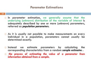
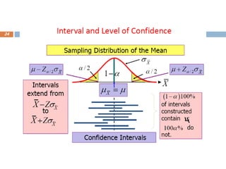
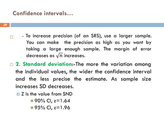
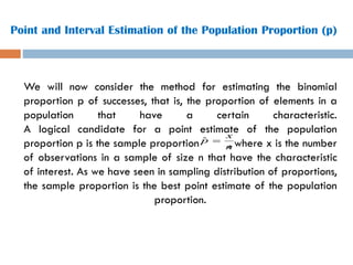
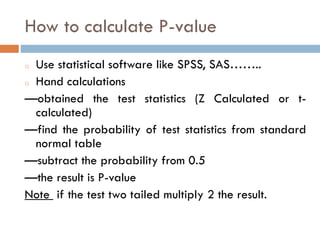
63. Hypothesis testing for single proportions
64
Example 7: In the study of childhood abuse in psychiatry patients, brown found
that 166 in a sample of 947 patients reported histories of physical or sexual abuse.
a) constructs 95% confidence interval
b) test the hypothesis that the true population proportion is 30%?
 Solution (a)
 The 95% CI for P is given by
]
2
.
0
;
151
.
0
[
0124
.
0
96
.
1
175
.
0
947
825
.
0
175
.
0
96
.
1
175
.
0
)
1
(
2








−


n
p
p
z
p 

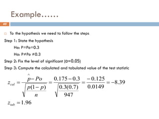
64. Example……
65
 To the hypothesis we need to follow the steps
Step 1: State the hypothesis
Ho: P=Po=0.3
Ha: P≠Po ≠0.3
Step 2: Fix the level of significant (α=0.05)
Step 3: Compute the calculated and tabulated value of the test statistic
96
.
1
39
.
8
0149
.
0
125
.
0
947
)
7
.
0
(
3
.
0
3
.
0
175
.
0
)
1
(
=
−
=
−
=
−
=
−
−
=

tab
cal
z
n
p
p
Po
p
z

65. Example……
66
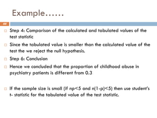
 Step 4: Comparison of the calculated and tabulated values of the
test statistic
 Since the tabulated value is smaller than the calculated value of the
test the we reject the null hypothesis.
 Step 6: Conclusion
 Hence we concluded that the proportion of childhood abuse in
psychiatry patients is different from 0.3
 If the sample size is small (if np<5 and n(1-p)<5) then use student’s
t- statistic for the tabulated value of the test statistic.

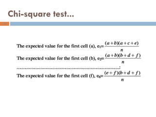
66. Chi-square test
 In recent years, the use of specialized statistical methods for
categorical data has increased dramatically, particularly for
applications in the biomedical and social sciences.
 Categorical scales occur frequently in the health sciences, for
measuring responses.
 E.g.
◼ patient survives an operation (yes, no),
◼ severity of an injury (none, mild, moderate, severe), and
◼ stage of a disease (initial, advanced).
 Studies often collect data on categorical variables that can be
summarized as a series of counts and commonly arranged in a
tabular format known as a contingency table
67

67. Chi-square Test Statistic cont’d…
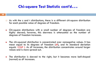
 As with the z and t distributions, there is a different chi-square distribution
for each possible value of degrees of freedom.
Chi-square distributions with a small number of degrees of freedom are
highly skewed; however, this skewness is attenuated as the number of
degrees of freedom increases.
The chi-squared distribution is concentrated over nonnegative values. It has
mean equal to its degrees of freedom (df), and its standard deviation
equals √(2df ). As df increases, the distribution concentrates around larger
values and is more spread out.
The distribution is skewed to the right, but it becomes more bell-shaped
(normal) as df increases.
68

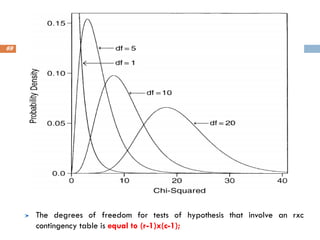
68. The degrees of freedom for tests of hypothesis that involve an rxc
contingency table is equal to (r-1)x(c-1);
69

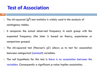
69. Test of Association
 The chi-squared (2) test statistics is widely used in the analysis of
contingency tables.
 It compares the actual observed frequency in each group with the
expected frequency (the later is based on theory, experience or
comparison groups).
 The chi-squared test (Pearson’s χ2) allows us to test for association
between categorical (nominal!) variables.
 The null hypothesis for this test is there is no association between the
variables. Consequently a significant p-value implies association.
70

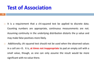
70. Test of Association
 It is a requirement that a chi-squared test be applied to discrete data.
Counting numbers are appropriate, continuous measurements are not.
Assuming continuity in the underlying distribution distorts the p value and
may make false positives more likely.
 Additionally, chi squared test should not be used when the observed values
in a cell are <5. It is, at times not inappropriate to pad an empty cell with a
small value, though, as one can only assume the result would be more
significant with no value there.
71

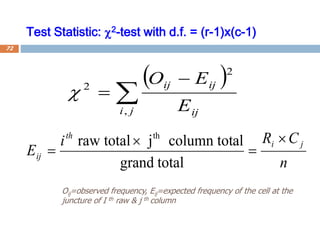
71. Test Statistic: 2-test with d.f. = (r-1)x(c-1)
( )

−
=
j
i ij
ij
ij
E
E
O
,
2
2

n
C
R
i
E
j
i
th
ij

=

=
total
grand
al
column tot
j
total
raw th
Oij=observed frequency, Eij=expected frequency of the cell at the
juncture of I th raw & j th column
72

72. Chi-square test...
73
Consider the following 3 by 2 contingency table

73. Chi-square test...
74

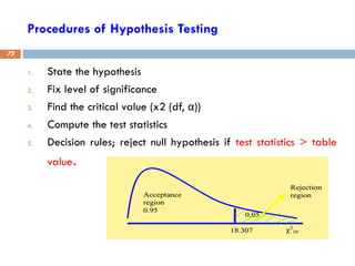
74. Procedures of Hypothesis Testing
1. State the hypothesis
2. Fix level of significance
3. Find the critical value (x2 (df, α))
4. Compute the test statistics
5. Decision rules; reject null hypothesis if test statistics > table
value.
75

75. Example 11:
Consider the following 3x2 contingency table
76

76. = 153.40
77
Chi-square test...

77. Right tail areas for the Chi-square Distribution
dfarea .995 .990 .975 .950 .900 .750 .500 .250 .100 .050 .025 .010 .005
1 0.00004 0.00016 0.00098 0.00393 0.01579 0.10153 0.45494 1.32330 2.70554 3.84146 5.02389 6.63490 7.87944
2 0.01003 0.02010 0.05064 0.10259 0.21072 0.57536 1.38629 2.77259 4.60517 5.99146 7.37776 9.21034 10.5966
3 0.07172 0.11483 0.21580 0.35185 0.58437 1.21253 2.36597 4.10834 6.25139 7.81473 9.34840 11.3448 12.8381
4 0.20699 0.29711 0.48442 0.71072 1.06362 1.92256 3.35669 5.38527 7.77944 9.48773 11.1432 13.2767 14.8602
5 0.41174 0.55430 0.83121 1.14548 1.61031 2.67460 4.35146 6.62568 9.23636 11.0705 12.8325 15.0862 16.7496
6 0.67573 0.87209 1.23734 1.63538 2.20413 3.45460 5.34812 7.84080 10.6446 12.5915 14.4493 16.811 18.5475
7 0.98926 1.23904 1.68987 2.16735 2.83311 4.25485 6.34581 9.03715 12.0170 14.0671 16.0127 18.4753 20.2777
8 1.34441 1.64650 2.17973 2.73264 3.48954 5.07064 7.34412 10.2188 13.3615 15.5073 17.5345 20.0902 21.9549
78
Chi-square table

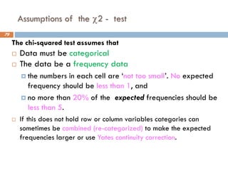
78. Assumptions of the 2 - test
The chi-squared test assumes that
 Data must be categorical
 The data be a frequency data
 the numbers in each cell are ‘not too small’. No expected
frequency should be less than 1, and
 no more than 20% of the expected frequencies should be
less than 5.
 If this does not hold row or column variables categories can
sometimes be combined (re-categorized) to make the expected
frequencies larger or use Yates continuity correction.
79

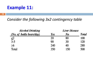
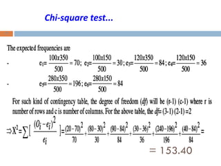
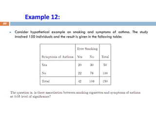
79. Example 12:
Consider hypothetical example on smoking and symptoms of asthma. The study
involved 150 individuals and the result is given in the following table:
80

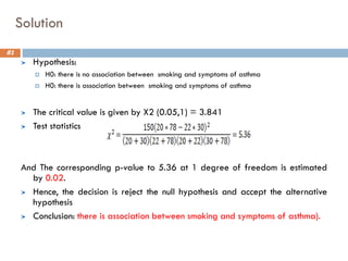
80. Solution
Hypothesis:
 H0: there is no association between smoking and symptoms of asthma
 H0: there is association between smoking and symptoms of asthma
The critical value is given by X2 (0.05,1) = 3.841
Test statistics
And The corresponding p-value to 5.36 at 1 degree of freedom is estimated
by 0.02.
Hence, the decision is reject the null hypothesis and accept the alternative
hypothesis
Conclusion: there is association between smoking and symptoms of asthma).
81

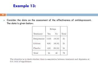
81. Example 13:
Consider the data on the assessment of the effectiveness of antidepressant.
The data is given below:
82

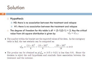
82. Solution
 Hypothesis
 H0: there is no association between the treatment and relapse
 H1: there is no association between the treatment and relapse
 The degree of freedom for this table is df = (3-1)(2-1) = 2. thus the critical
value from chi-square distribution is given by = 9.21
83

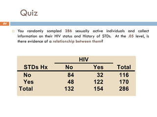
83. Quiz
 You randomly sampled 286 sexually active individuals and collect
information on their HIV status and History of STDs. At the .05 level, is
there evidence of a relationship between them?
84
HIV
STDs Hx No Yes Total
No 84 32 116
Yes 48 122 170
Total 132 154 286

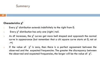
84. Summery
Characteristics χ2
1. Every χ2 distribution extends indefinitely to the right from 0.
2. Every χ2 distribution has only one (right ) tail.
3. As df increases, the χ2 curves get more bell shaped and approach the normal
curve in appearance (but remember that a chi square curve starts at 0, not at
-∞)
4. If the value of χ2 is zero, then there is a perfect agreement between the
observed and the expected frequencies. The greater the discrepancy between
the observed and expected frequencies, the larger will be the value of χ2.
85