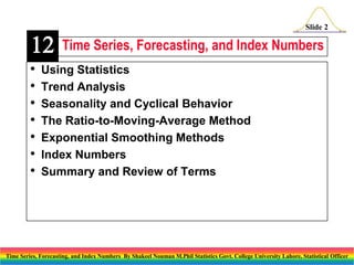
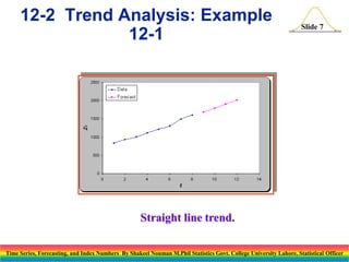
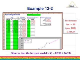
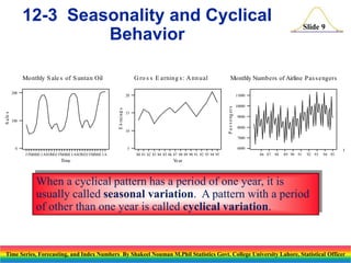
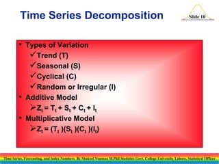
GIÁO ÁN DẠY THÊM (KẾ HOẠCH BÀI BUỔI 2) - TIẾNG ANH 8 GLOBAL SUCCESS (2 CỘT) N...
Time series, forecasting, and index numbers
1. Time Series, Forecasting, and Index
Numbers
Slide 1
Shakeel Nouman
M.Phil Statistics
Time Series, Forecasting, and Index Numbers By Shakeel Nouman M.Phil Statistics Govt. College University Lahore, Statistical Officer
2. 12
Slide 2
Time Series, Forecasting, and Index Numbers
• Using Statistics
• Trend Analysis
• Seasonality and Cyclical Behavior
• The Ratio-to-Moving-Average Method
• Exponential Smoothing Methods
• Index Numbers
• Summary and Review of Terms
Time Series, Forecasting, and Index Numbers By Shakeel Nouman M.Phil Statistics Govt. College University Lahore, Statistical Officer
3. 12-1 Using Statistics
Slide 3
A time series is a set of measurements of a variable that are ordered
through time. Time series analysis attempts to detect and
understand regularity in the fluctuation of data over time.
Regular movement of time series data may result from a tendency
to increase or decrease through time - trend- or from a tendency to
follow some cyclical pattern through time - seasonality or cyclical
variation.
Forecasting is the extrapolation of series values beyond the region
of the estimation data. Regular variation of a time series can be
forecast, while random variation cannot.
Time Series, Forecasting, and Index Numbers By Shakeel Nouman M.Phil Statistics Govt. College University Lahore, Statistical Officer
4. The Random Walk
Slide 4
A random walk:
Zt- Zt-1=at
or equivalently:
Zt= Zt-1+at
The difference between Z in time t and time t-1 is a random error.
R andom W alk
15
10
5
Z
0
There is no evident regularity in a
random walk, since the difference in the
series from period to period is a random
error. A random walk is not
forecastable.
a
0
10
20
30
40
50
t
Time Series, Forecasting, and Index Numbers By Shakeel Nouman M.Phil Statistics Govt. College University Lahore, Statistical Officer
5. A Time Series as a
Superposition of Cyclical
Functions
Slide 5
A Time Series as a Superposition of Two Wave
Functions and a Random Error (not shown)
z
4
3
2
1
0
-1
0
10
20
30
40
50
t
In contrast with a random walk, this series exhibits obvious
cyclical fluctuation. The underlying cyclical series - the
regular elements of the overall fluctuation - may be analyzable
and forecastable.
Time Series, Forecasting, and Index Numbers By Shakeel Nouman M.Phil Statistics Govt. College University Lahore, Statistical Officer
6. 12-2 Trend Analysis: Example
12-1
Slide 6
The following output was obtained using the template.
Zt = 696.89 + 109.19t
Note: The template contains forecasts for t = 9 to t = 20 which corresponds to years 2002 to 2013.
Time Series, Forecasting, and Index Numbers By Shakeel Nouman M.Phil Statistics Govt. College University Lahore, Statistical Officer
7. 12-2 Trend Analysis: Example
12-1
Slide 7
Straight line trend.
Time Series, Forecasting, and Index Numbers By Shakeel Nouman M.Phil Statistics Govt. College University Lahore, Statistical Officer
8. Example 12-2
Slide 8
The forecast
for t = 10
(year 2002)
is 345.27
Observe that the forecast model is Zt = 82.96 + 26.23t
Time Series, Forecasting, and Index Numbers By Shakeel Nouman M.Phil Statistics Govt. College University Lahore, Statistical Officer
9. 12-3 Seasonality and Cyclical
Behavior
G ro s s E arning s : A nn ual
Monthly S ale s of S untan Oil
Monthly Numbers of Airline P as s engers
20
100
11000
P a s s e ng er s
E a rnin g s
S a le s
200
Slide 9
15
10
10000
9000
8000
7000
0
6000
5
J FMAMJ J AS OND J FMAMJ J ASOND J FMAMJ J A
80 81 82 83 84 85 86 87 88 89 90 91 92 93 94 95
Time
t
86 87
88
89 90 91
92 93
94 95
Ye ar
When a cyclical pattern has a period of one year, it is
usually called seasonal variation. A pattern with a period
of other than one year is called cyclical variation.
Time Series, Forecasting, and Index Numbers By Shakeel Nouman M.Phil Statistics Govt. College University Lahore, Statistical Officer
10. Time Series Decomposition
•
•
•
Slide 10
Types of Variation
Trend (T)
Seasonal (S)
Cyclical (C)
Random or Irregular (I)
Additive Model
Zt = Tt + St + Ct + It
Multiplicative Model
Zt = (Tt )(St )(Ct )(It)
Time Series, Forecasting, and Index Numbers By Shakeel Nouman M.Phil Statistics Govt. College University Lahore, Statistical Officer
11. Estimating an Additive Model
with Seasonality
Slide 11
An additive regression model with seasonality:
Zt=0+ 1 t+ 2 Q1+ 3 Q2 + 4 Q3 + at
where
Q1=1 if the observation is in the first quarter, and 0
otherwise
Q2=1 if the observation is in the second quarter,
and 0 otherwise
Q3=1 if the observation is in the third quarter, and
0 otherwise
Time Series, Forecasting, and Index Numbers By Shakeel Nouman M.Phil Statistics Govt. College University Lahore, Statistical Officer
12. 12-4 The Ratio-to-MovingAverage Method
Slide 12
A moving average of a time series is an average of a fixed
number of observations that moves as we progress down the
series.
Time, t:
Series, Zt:
1
15
2
12
3
11
4
18
6
7
8
9 10
11
12
13
16
14
17 20 18
21
16
14
Five-period
15.4 15.6 16.0 17.2 17.6 17.0 18.0 18.4 17.8 17.6
14
19
3
11
4
18
14
19
moving average:
Time, t:
Series, Zt:
1
15
2
12
5
21
5
6
7
8
9 10
11
12
21
16
14
17 20 18
21
16
(15 + 12 + 11 + 18 + 21)/5=15.4
(12 + 11 + 18 + 21 + 16)/5=15.6
(11 + 18 + 21 + 16 + 14)/5=16.0
13
14
. . . . .
(18 + 21 + 16 + 14 + 19)/5=17.6
Time Series, Forecasting, and Index Numbers By Shakeel Nouman M.Phil Statistics Govt. College University Lahore, Statistical Officer
13. Comparing Original Data and
Smoothed Moving Average
Original Series and Five-Period Moving Averages
•
Slide 13
Moving Average:
– “Smoother”
– Shorter
– Deseasonalized
20
Z
– Removes seasonal and
irregular components
15
– Leaves trend and
cyclical components
10
0
5
10
15
t
Z
t TSCI SI
MA TC
Time Series, Forecasting, and Index Numbers By Shakeel Nouman M.Phil Statistics Govt. College University Lahore, Statistical Officer
14. Ratio-to-Moving Average
•
Slide 14
Ratio-to-Moving Average for Quarterly Data
Compute a four-quarter moving-average
series.
Center the moving averages by averaging
every consecutive pair and placing the average
between quarters.
Divide the original series by the corresponding
moving average. Then multiply by 100.
Derive quarterly indexes by averaging all data
points corresponding to each quarter. Multiply
each by 400 and divide by sum.
Time Series, Forecasting, and Index Numbers By Shakeel Nouman M.Phil Statistics Govt. College University Lahore, Statistical Officer
15. Ratio-to-Moving Average:
Example 12-3
Ratio
to Moving
Average
*
*
93.3
100.9
110.2
93.8
90.1
107.5
106.4
100.7
90.5
95.0
113.9
97.9
*
*
Four-Quarter Moving Averages
Actual
Smoothed
Actual
Smoothed
170
160
Sales
Quarter
1998W
1998S
1998S
1998F
1999W
1999S
1999S
1999F
2000W
2000S
2000S
2000F
2002W
2002S
2002S
2002F
Simple
Centered
Moving
Moving
Sales Average
Average
170
*
*
148
*
*
141
*
151.125
150
152.25
148.625
161
150.00
146.125
137
147.25
146.000
132
145.00
146.500
158
147.00
147.000
157
146.00
147.500
145
148.00
144.000
128
147.00
141.375
134
141.00
141.000
160
141.75
140.500
139
140.25
142.000
130
140.75
*
144
143.25
*
Slide 15
150
Moving Average
Length:
4
140
MAPE:
MAD:
MSD:
130
0
5
10
7.816
10.955
152.574
15
T
ime
Time Series, Forecasting, and Index Numbers By Shakeel Nouman M.Phil Statistics Govt. College University Lahore, Statistical Officer
16. Seasonal Indexes: Example 12-3
Year
Winter
1998
1999
2000
Quarter
Spring
Summer
110.2
106.4
2002
Sum
Average
93.8
100.7
113.9
93.3
90.1
90.5
97.9
330.5
110.17
292.4
97.47
273.9
91.3
Slide 16
Fall
100.9
107.5
95.0
303.4
101.13
Sum of Averages = 400.07
Seasonal Index = (Average)(400)/400.07
Index
110.15
Seasonal
97.45
91.28
101.11
Time Series, Forecasting, and Index Numbers By Shakeel Nouman M.Phil Statistics Govt. College University Lahore, Statistical Officer
17. Deseasonalized Series: Example
12-3
Original and SeasonallyAdjusted Series
170
160
Sales
Seasonal
Deseasonalized
Quarter
Sales
Index (S)
Series(Z/S)*100
1998W
170
110.15
154.34
1998S
148
97.45
151.87
1998S
141
91.28
154.47
1998F
150
101.11
148.35
1999W
161
110.15
146.16
1999S
137
97.45
140.58
1999S
132
91.28
144.51
1999F
158
101.11
156.27
2000W
157
110.15
142.53
2000S
145
97.45
148.79
2000S
128
91.28
140.23
2000F
134
101.11
132.53
2002W
160
110.15
145.26
2002S
139
97.45
142.64
2002S
130
91.28
142.42
2002F
144
101.11
142.42
Slide 17
150
140
130
1992W
1992S
1992S
1992F
t
Original
Deseasonalized - - -
Time Series, Forecasting, and Index Numbers By Shakeel Nouman M.Phil Statistics Govt. College
University Lahore, Statistical Officer
18. The Cyclical Component:
Example 12-3
Trend Line and Moving Averages
180
Sales
170
160
150
140
130
120
1992W
1992S
1992S
t
1992F
Slide 18
The cyclical component is
the remainder after the
moving averages have been
detrended. In this example,
a comparison of the moving
averages and the estimated
regression line:
Z 155.275 11059 t
.
illustrates that the cyclical
component in this series is
negligible.
Time Series, Forecasting, and Index Numbers By Shakeel Nouman M.Phil Statistics Govt. College University Lahore, Statistical Officer
19. Example 12-3 using the
Template
Slide 19
The centered moving average, ratio to moving average, seasonal index, and deseasonalized
values were determined using the Ratio-to-Moving-Average method.
This displays just
a partial output
for the quarterly
forecasts.
Time Series, Forecasting, and Index Numbers By Shakeel Nouman M.Phil Statistics Govt. College University Lahore, Statistical Officer
20. Example 12-3 using the
Template
Slide 20
Graph of the quarterly Seasonal
Index
Time Series, Forecasting, and Index Numbers By Shakeel Nouman M.Phil Statistics Govt. College University Lahore, Statistical Officer
21. Example 12-3 using the
Template
Slide 21
Graph of the Data and the quarterly Forecasted values
Time Series, Forecasting, and Index Numbers By Shakeel Nouman M.Phil Statistics Govt. College University Lahore, Statistical Officer
22. Example 12-3 using the
Template
Slide 22
The centered moving average, ratio to moving average, seasonal index, and deseasonalized
values were determined using the Ratio-to-Moving-Average method.
This displays just
a partial output
for the monthly
forecasts.
Time Series, Forecasting, and Index Numbers By Shakeel Nouman M.Phil Statistics Govt. College University Lahore, Statistical Officer
23. Example 12-3 using the
Template
Slide 23
Graph of the monthly Seasonal Index
Time Series, Forecasting, and Index Numbers By Shakeel Nouman M.Phil Statistics Govt. College University Lahore, Statistical Officer
24. Example 12-3 using the
Template
Slide 24
Graph of the Data and the monthly Forecasted values
Time Series, Forecasting, and Index Numbers By Shakeel Nouman M.Phil Statistics Govt. College University Lahore, Statistical Officer
25. Forecasting a Multiplicative
Series: Example 12-3
Slide 25
The forecast of a multiplicative series :
ˆ
Z = TSC
Forecast for Winter 2002 (t = 17) :
Trend : z = 152.26 - (0.837)(17) = 138.03
ˆ
S = 1.1015
C 1 (negligibl e)
ˆ
Z = TSC
= (1)(138.03)(1.1015) = 152.02
Time Series, Forecasting, and Index Numbers By Shakeel Nouman M.Phil Statistics Govt. College University Lahore, Statistical Officer
26. Multiplicative Series: Review
Slide 26
Z ( Trend )( Seasonal ( Cyclical )( Irregular )
TSCI
MA ( Trend )( Cyclical )
TC
Z
TSCI
SI
MA
TC
S = Average of SI (Ratio - to - Moving Averages)
Z
TSCI
CTI (Deseasonalized Data)
S
S
Time Series, Forecasting, and Index Numbers By Shakeel Nouman M.Phil Statistics Govt. College University Lahore, Statistical Officer
27. 12-5 Exponential Smoothing
Methods
Slide 27
Smoothing is used to forecast a series by first removing sharp
variation, as does the moving average.
Weights Decline as we go back in
Time
Weights Decline as We Go Back in Time and Sum to 1
W e ig ht
Weight
0.4
0.3
0.2
0.1
0.0
-15
-10
-5
Exponential smoothing is a forecasting
method in which the forecast is based in
a weighted average of current and past
series values. The largest weight is
given to the present observations, less
weight to the immediately preceding
observation, even less weight to the
observation before that, and so on. The
weights decline geometrically as we go
back in time.
0
Lag
-10
Lag
0
Time Series, Forecasting, and Index Numbers By Shakeel Nouman M.Phil Statistics Govt. College University Lahore, Statistical Officer
28. The Exponential Smoothing
Model
Slide 28
Given a weighting factor: 0 < w < 1:
2
3
Z t 1 w ( Z t ) w (1 w )( Z t 1 ) w (1 w ) ( Z t 2 ) w (1 w ) ( Z t 3 )
Since
2
3
Z t w ( Z t 1 ) w (1 w )( Z t 2 ) w (1 w ) ( Z t 3 ) w (1 w ) ( Z t 4 )
2
3
(1 w ) Z t w (1 w )( Z t 1 ) w (1 w ) ( Z t 2 ) w (1 w ) ( Z t 3 )
So
Z t 1 w(Z t ) (1 w)(Z t )
Z t 1 Z t (1 w)(Z t - Z t )
Time Series, Forecasting, and Index Numbers By Shakeel Nouman M.Phil Statistics Govt. College University Lahore, Statistical Officer
30. Example 12-4 – Using the
Template
Slide 30
Time Series, Forecasting, and Index Numbers By Shakeel Nouman M.Phil Statistics Govt. College University Lahore, Statistical Officer
31. 12-6 Index Numbers
Slide 31
An index number is a number that measures the relative
change in a set of measurements over time. For example: the
Dow Jones Industrial Average (DJIA), the Consumer Price
Index (CPI), the New York Stock Exchange (NYSE) Index.
Value in period i
Index number in period i: = 100
Value in base period
Changing the base period of an index:
Old index value
New index value: = 100
Index value of new base
Time Series, Forecasting, and Index Numbers By Shakeel Nouman M.Phil Statistics Govt. College University Lahore, Statistical Officer
32. Index Numbers: Example 12-5
Pric e and Index (1982=100) of Natural Gas Price
Index
Index
Year Price 1984-Base 1991-Base
121
121
133
146
162
164
172
187
197
224
255
247
238
222
100.0
100.0
109.9
120.7
133.9
135.5
142.1
154.5
162.8
185.1
210.7
204.1
196.7
183.5
64.7
64.7
71.1
78.1
86.6
87.7
92.0
100.0
105.3
119.8
136.4
132.1
127.3
118.7
250
Original
P ric e
1984
1985
1986
1987
1988
1989
1990
1991
1992
1993
1994
1995
1996
1997
Slide 32
Index (1984)
150
Index (1991)
50
1985
1990
1995
Ye ar
Time Series, Forecasting, and Index Numbers By Shakeel Nouman M.Phil Statistics Govt. College University Lahore, Statistical Officer
33. Consumer Price Index –
Example 12-6
Consumer Price index (CPI): 1967=100
Slide 33
Example 12-6:
450
CPI
350
250
150
50
1950 1955 1960 1965 1970 1975 1980 1985 1990 1995
Ye a r
Salary
Adjusted Salary =
100
CPI
Adjusted
Year
Salary Salary
1980
29500 11953.0
1981
31000 11380.3
1982
33600 11610.2
1983
35000 11729.2
1984
36700 11796.8
1985
38000 11793.9
Time Series, Forecasting, and Index Numbers By Shakeel Nouman M.Phil Statistics Govt. College University Lahore, Statistical Officer
34. Example 12-6: Using the
Template
Slide 34
Time Series, Forecasting, and Index Numbers By Shakeel Nouman M.Phil Statistics Govt. College University Lahore, Statistical Officer
35. Slide 35
Name
Religion
Domicile
Contact #
E.Mail
M.Phil (Statistics)
Shakeel Nouman
Christian
Punjab (Lahore)
0332-4462527. 0321-9898767
sn_gcu@yahoo.com
sn_gcu@hotmail.com
GC University, .
(Degree awarded by GC University)
M.Sc (Statistics)
Statitical Officer
(BS-17)
(Economics & Marketing
Division)
GC University, .
(Degree awarded by GC University)
Livestock Production Research Institute
Bahadurnagar (Okara), Livestock & Dairy Development
Department, Govt. of Punjab
Time Series, Forecasting, and Index Numbers By Shakeel Nouman M.Phil Statistics Govt. College University Lahore, Statistical Officer