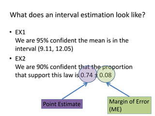
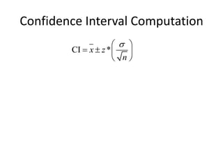
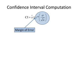
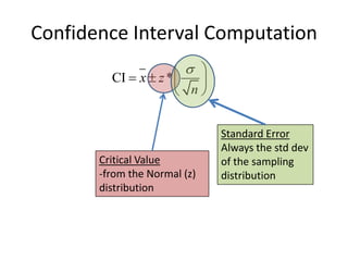
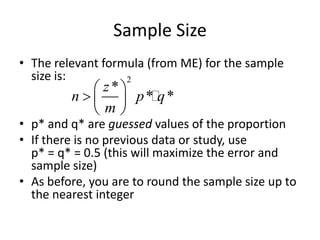
This document provides an overview of confidence intervals. It defines key terms like statistical inference, confidence level, and margin of error. It explains how to construct confidence intervals for means using the z-distribution when the population standard deviation is known, and using the t-distribution when it is unknown. It also covers how to estimate population proportions using the normal distribution. Examples are provided to demonstrate how to use the PANIC method to set up and calculate confidence intervals.

1. Chapter 10Estimating with Confidence

2. 10.1 Confidence Intervals: The Basics

3. DefinitionsStatistical InferenceThe method of drawing conclusions about a population based on a sampleThe last Major Topic for this last statistics courseThe mindset: we are looking at data that comes from a random sample (or an experiment) and inferring characteristics of the population

4. The Basic Plan In the absence of other data, the sample estimate is the estimate of the parameterWe would like an interval estimationState the parameter that is being estimatedCheck to see if the data can be NormalizedCompute the interval using area under the Normal curveWrite a nice conclusion

5. What does an interval estimation look like?EX1We are 95% confident the mean is in the interval (9.11, 12.05)

6. What does an interval estimation look like?EX1We are 95% confident the mean is in the interval (9.11, 12.05)Confidence Level C

7. What does an interval estimation look like?EX1We are 95% confident the mean is in the interval (9.11, 12.05)Confidence Interval(CI)

8. What does an interval estimation look like?EX1We are 95% confident the mean is in the interval (9.11, 12.05)Lower BoundUpper Bound

9. What does an interval estimation look like?EX1We are 95% confident the mean is in the interval (9.11, 12.05)EX2We are 90% confident that the proportion that support this law is 0.74 ± 0.08

10. What does an interval estimation look like?EX1We are 95% confident the mean is in the interval (9.11, 12.05)EX2We are 90% confident that the proportion that support this law is 0.74 ± 0.08Confidence Level C

11. What does an interval estimation look like?EX1We are 95% confident the mean is in the interval (9.11, 12.05)EX2We are 90% confident that the proportion that support this law is 0.74 ± 0.08Confidence Interval (CI)

12. What does an interval estimation look like?EX1We are 95% confident the mean is in the interval (9.11, 12.05)EX2We are 90% confident that the proportion that support this law is 0.74 ± 0.08Margin of Error(ME)Point Estimate

13. Confidence LevelThe value of the parameter is fixed before we start our samplingEither the parameter is ‘in’ our interval or it’s not.There is no probability involved here“There is a 95% probability the parameter is in the interval”

14. Confidence LevelThe value of the parameter is fixed before we start our samplingEither the parameter is ‘in’ our interval or it’s not.There is no probability involved here“There is a 95% probability the parameter is in the interval”F A I L

15. Confidence LevelRemember that our sample is just one of many samples that could have been takenIf good sampling technique is used, 95% (for example) of the samples would contain the parameterWe just don’t know if our sample is part of the 95% or the 5%

16. Confidence LevelInterpretation of “90% Confidence Level”“We are 90% confident that our CI contains the value of the parameter”“90% of CI’s computed with this technique will contain the parameter”“There is a 90% probability our CI contains the parameter”WRONG INTERPRETATION

17. Confidence LevelInterpretation of “90% Confidence Level”“We are 90% confident that our CI contains the value of the parameter”“90% of CI’s computed with this technique will contain the parameter”“There is a 90% probability our CI contains the parameter”WRONG INTERPRETATION

18. PANICWhen constructing Confidence Intervals for the AP test, there is a definite checklist that readers look forUse the acronym P.A.N.I.C. to help memorize the steps to construction a confidence intervalP = state the ParameterA = check that Assumptions are satisfiedN = state is the Name of the intervalI = compute numerical values of the IntervalC = write a Conclusion for your findings

19. PANIC for MeansWe are going to start with Means, we’ll save proportions for laterParameterdefine what  measuresdefine what x-bar measures“ = mean length of all Great White Sharks‘ flukesx-bar = mean length the Great White Shark flukes in our sample of 35 sharks”

20. Assumptions for CI’s of MeanSRS- the data must have come from an SRSIndependence- the population size must be more than 10 times the sampleN> 10n (Independence)

21. Assumptions for CI’s of MeanSRS- the data must have come from an SRSIndependence- the population size must be more than 10 times the sampleN> 10n (Independence)This is a condition that must be met since we are sampling without replacement and our formula forstd dev needs to hold true

22. Assumptions for CI’s of MeanSRS- the data must have come from an SRSIndependence- the population size must be more than 10 times the sampleN> 10n (Independence)The sampling Distribution is approximately Normal (Normality)

23. More on NormalityWe are looking for justification that the sampling distribution is NormalIf the population is Normal, then the samp dist is also NormalIf n> 30 and the sample data is not given, state “The Central Limit Theorem guarantees that the sampling distribution is Normal”For smaller samples, check the following:(1) the Histogram is single peak, symmetric with no outliers(2) the Normal Probability Plot is approx Linear

24. Name of the IntervalCurrently, the only Interval we will worry about is “z-interval for sample means”This will always be the name of the distribution used

25. Confidence Interval Computation

26. Confidence Interval ComputationMargin of Error

27. Confidence Interval ComputationStandard ErrorAlways the std devof the sampling distributionCritical Value-from the Normal (z) distribution

28. Critical ValueThe area between –z* and +z* = Confidence LevelBecause they are used frequently, there is a shorthand method in table CThe last row gives different confidence levelsKeep critical values to 3 decimal places The row above the CL row has the z*In the AP test, they will call this z

29. A General z* curve

30. z* for a 80% CL

31. Computing a CILet’s compute the 95% CI for a sample of 35, with a mean of 5.38 and a population std dev =0.74(1) locate the critical valuez* = 1.960(2) Compute S.E. and M.E.SE = 0.74/(35) = 0.1251ME = (1.960)(0.1251) = 0.2452

32. Computing a CIState the CI = 5.38 ± 0.25Interval estimate:(5.13, 5.63)Notice that the point estimate is the average of the upper and lower bounds

33. ConclusionsWe are 95% confident that the mean length of a great white shark fluke is 5.38 ± 0.25 ft. ORWe are 95% confident that the mean length of all great white shark flukes is in the interval (5.13 ft, 5.63 ft).

34. Calculators TI83/TI84

35. Calculators TI83/TI84Your TI is very efficient for finding these intervals! This doesn’t excuse you from the mathematics, of course.[stat] -> “TESTS” -> “Zinterval”Inpt: “Stats” (if your data is in L1, you can use “Data”Enter values for , x-bar, n, and C-Level.Viola!

36. Calculators TI89Run the “Stats/List Editor” APP[2nd] -> [F2] (F7) -> “Zinterval”Input Method = “Stats”Choose Data if all the observations are in a ListEnter values for , x-bar, n, and C-Level.Viola!

37. Behavior of Margin of ErrorME = z* (/n)In practice, we would like to minimize ME.(1) decrease z* This also means decrease our CL!(2) increase nthis is usually a trade off, since obtaining large samples could be more expensive/time consuming(3) decrease Not really an option.  is a known quantity.

38. Sample SizeBy using algebra, we can get a formula to compute minimum sample size for a given MEYou should always round the sample size up in this calculationNote: ME is produced by sampling variability, it has nothing to do with “sloppy work”

39. 10.2 Estimating a Population Mean

40. Student’s t-distributionThe confidence intervals computed in the previous section assumed that we knew .It doesn’t seem likely that we would know  and not know the value of When  is unknown, we can no longer use the Normal distribution

41. Student’s t-distributionThe t-distribution is to be used when  is unknown.The t-distribution is very similar to the Normal distribution with a key differenceThe shape of the distribution changes based upon the sample size/degrees of freedom (df)Large samples have a tall peak and thinner tailsSmall samples have a small peak and thicker tails.

42. Student’s t-distributionDegrees of Freedom = n -1

43. Using the t-distributionThe CI is found using PANICThe Assumptions are the same as a z-intervalSince sample sizes tend to be small, you will most likely need to check the histogram (symmetric, no outliers) and Normal prob plot (approx linear)We cannot use the t-distribution when there are outliers!The Name of the interval is “1-sample t-interval for mean”

44. Using the t-distributionInterval is computed withdf = n – 1t* is from table C or your calculators is the sample’s standard deviationUses the sample std dev to approximate 

45. Upper Tail Area

46. Upper Tail AreaThis is the Upper Tail Area

47. Using the t-distribution

48. Using the t-distributionUsing TI84 [2nd] -> [vars](DIST) -> “invT”“invT(1-Upper Tail Area, df)”Where “Upper Tail Area” = (1-CL)/2This is the area to the left of the right crit. Value.ALTERNATIVELY, you may use“−invT(Upper Tail Area, df)”

49. Using the t-distributionUsing TI84 [2nd] -> [vars](DIST) -> “invT”“invT(1-Upper Tail Area, df)”Where “Upper Tail Area” = (1-CL)/2This is the area to the left of the right crit. Value.ALTERNATIVELY, you may use“−invT(Upper Tail Area, df)”

50. Using the t-distributionUsing TI84 [2nd] -> [vars](DIST) -> “invT”“invT(1-Upper Tail Area, df)”Where “Upper Tail Area” = (1-CL)/2This is the area to the left of the right crit. Value.ALTERNATIVELY, you may use“−invT(Upper Tail Area, df)”Don’t forget the negative!

51. Using the t-distribution

52. Using the t-distributionUsing TI89From home screen:[catalog] -> [F3](FlashApps) -> inv_t…TIStat“tistat.invT(1-Upper Tail Area, df)”Where “Upper Tail Area” = (1-CL)/2This is the area to the left of the right crit. Value.ALTERNATIVELY, you may use“-tistat.invT(Upper Tail Area, df)”

53. Using the t-distributionUsing TI89From home screen:[catalog] -> [F3](FlashApps) -> inv_t…TIStat“tistat.invT(1-Upper Tail Area, df)”Where “Upper Tail Area” = (1-CL)/2This is the area to the left of the right crit. Value.ALTERNATIVELY, you may use“-tistat.invT(Upper Tail Area, df)”

54. Using the t-distributionUsing TI89From home screen:[catalog] -> [F3](FlashApps) -> inv_t…TIStat“tistat.invT(1-Upper Tail Area, df)”Where “Upper Tail Area” = (1-CL)/2This is the area to the left of the right crit. Value.ALTERNATIVELY, you may use“-tistat.invT(Upper Tail Area, df)”Don’t forget the negative!

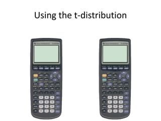
55. Using the t-distributionALTERNATIVE TI89 titanium[APPS] -> “Stat/List Editor” -> [F5] (distrib) -> “Inverse” -> “Inverse t…” “Area: 1- Upper Tail”Upper Tail = (1 – CL)/2“degrees of freedom, df: df”This takes longer to get to, but the menu “guides” you through

56. Table COccasionally, you will need to fine the t* for a df that does not appear in the chart.When this happens, you are to use the nearest greatest df in the same columnThis usually means “use the t* that is in the line above where the desired t* should be”

57. Example: 1 sample t-interval Problem 10.30 The amount of Vitamin C (mg/100g) in CSB for a random sample of 8 are given as: 26, 31, 23, 22, 11, 22, 14, 31 Construct a 95% Confidence interval for the amount of vitamin C in CSB.

58. Example: 1 sample t-intervalParameter = the mean amount of vitamin C in CSB produced at the factoryx-bar = the mean amount of vitamin C in a sample n = 8

59. Example: 1 sample t-intervalAssumptionsSRS‘Our problem states that we have a random sample’Independence‘10n = 80 < N; we can infer that more than 80 CSB is produced in the factory’

60. Example: 1 sample t-intervalAssumptionsNormality‘The histogram is symmetric w/ no outliers’‘The Norm Prob Plot is approx linear’‘We have good evidence that our sampling distribution is approximately Normal’x10 15 20 25 30 35Norm Prob PlotHistogramz

61. Example: 1 sample t-intervalName of Interval ‘We will compute a 1-sample t-interval for a mean’

62. Example: 1 sample t-intervalName of Interval ‘We will compute a 1-sample t-interval for a mean’Interval Calculation

63. Example: 1 sample t-intervalName of Interval ‘We will compute a 1-sample t-interval for a mean’Interval CalculationConclusion ‘We are 95% confident that the mean amount of vitamin C in a unit of CSB produced in the factory is between 16.487 and 28.513 mg/100 g’

64. 10.3 Estimating a population Proportion

65. Estimating a ProportionLike with means, we are going to estimate the population proportion based on the proportion in a samplex = # of positive responsesn = total number of responsesWe will again use the PANIC proceduresNote: nothing is averaged. We are not looking at the average proportion from many samples

66. ParameterSome typical parameters:‘p = prop of people in CA who support the proposition p-hat = proportion of people in a sample n = 35 who support the proposition’‘p = prop of students at THS who ride the bus p-hat = propotion of students in a sample (n = 14) from THS who ride the bus

67. AssumptionsSimple Random Sample SRS must be either stated or inferredIndependencebecause you are usually sampling without replacement:N> 10nNormalityn·p-hat > 10n·q-hat > 10

68. Name of the Interval“1-proportion z interval”Unlike for means, you will always use the Normal curve when dealing with proportions!

69. Interval Calculationz* is calculated as beforeUse table C OR“ − invNorm( (1 – C) /2 )”This calculation is similar to the calculations for the last section

70. Interval Calculationz* is calculated as beforeUse table C OR“ − invNorm( (1 – C) /2 )”This calculation is similar to the calculations for the last sectionMargin of Error (ME)

71. Interval Calculationz* is calculated as beforeUse table C OR“ − invNorm( (1 – C) /2 )”This calculation is similar to the calculations for the last sectionStandard Error(SE)

72. ConclusionSome Examples:We are 90% confident that the proportion of voters in CA who support the proposition is 0.34 ± 0.03We are 95% confident that the proportion of students at THS who ride this bus is in the interval (0.39, 0.44)

73. Sample SizeThe relevant formula (from ME) for the sample size is:p* and q* are guessed values of the proportionIf there is no previous data or study, use p* = q* = 0.5 (this will maximize the error and sample size)As before, you are to round the sample size up to the nearest integer

74. TI83/84

75. TI83/84[stat] -> “TEST” -> “1-PropZInt”“x: number of successes” this can be computed with “p-hat x n”“n: number of people in sample”“C-Level : confidence level”“Calculate” and you are doneYou still need to fully write up “PANIC” procedures

76. TI 89

77. TI 89[APPS] -> “Stat/List Editor”[2nd] -> [F2](F7) -> “1-PropZInt”“Successes x: # of successes”“n: number of people in sample”“C-Level : confidence level”“Calculate” and you are doneYou still need to fully write up “PANIC” procedures

78. Example 1-PropZInt The 2004 Gallup Youth Survey asked a random sample of 439 US teens aged 13 to 17 whether they though young people should wait to have sex until marriage. 246 sad “yes.” Let’s construct a 95% confidence interval for the proportion of all teens who would say “Yes”

79. Parameterp = the proportion of all teens in the US aged 13-17 who would answer “Yes” to the surveyp-hat = the proportion of teens in the survey of 439 who answered “Yes” to the survey

80. AssumptionsSRS: We are told in the problem that the survey was random sample.Independence: there are than 10(439) = 4390 teens aged 13-17 in the USNormalityn x p-hat = 246, n x q-hat = 193The sampling distribution is approx. Normal(Note that this is just #successes and #failures)

81. Name of IntervalWe are constructing a “1 proportion Z interval”

82. Construction of Interval

83. Conclusion“We are 95% confident that the true proportion of 13-17 year olds who would answer “yes” when asked if young people should wait to have sex until they are married is between 0.514 and 0.606.”