Contingency Tables

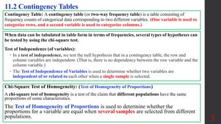
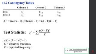
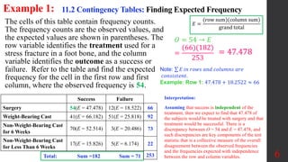
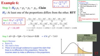
Elementary Statistics
Chapter 11:
Goodness-of-Fit and
Contingency Tables
11.2 Contingency Tables
1

Chapter 11:
Goodness-of-Fit and Contingency Tables
11.1 Goodness-of-Fit
2
Objectives:
1 Test a distribution for goodness of fit, using chi-square.
2 Test two variables for independence, using chi-square.
3 Test proportions for homogeneity, using chi-square.

3
Contingency Table: A contingency table (or two-way frequency table) is a table consisting of
frequency counts of categorical data corresponding to two different variables. (One variable is used to
categorize rows, and a second variable is used to categorize columns.)
When data can be tabulated in table form in terms of frequencies, several types of hypotheses can
be tested by using the chi-square test.
Test of Independence (of variables):
 In a test of independence, we test the null hypothesis that in a contingency table, the row and
column variables are independent. (That is, there is no dependency between the row variable and the
column variable.)
 The Test of Independence of Variables is used to determine whether two variables are
independent of or related to each other when a single sample is selected.
Chi-Square Test of Homogeneity: (Test of Homogeneity of Proportions)
A chi-square test of homogeneity is a test of the claim that different populations have the same
proportions of some characteristics.
The Test of Homogeneity of Proportions is used to determine whether the
proportions for a variable are equal when several samples are selected from different
populations.

4
11.2 Contingency Tables Objective, Notation & Requirements
Conduct a hypothesis test of independence between the row variable and column variable in a contingency table.
O represents the observed frequency in a cell of a contingency table.
E represents the expected frequency in a cell, found by assuming that the row and column variables are
independent.
r represents the number of rows in a contingency table (not including labels or row totals).
c represents the number of columns in a contingency table (not including labels or column totals).
Requirements
1. The sample data are randomly selected.
2. The sample data are represented as frequency counts in a two-way table.
3. For every cell in the contingency table, the expected frequency E is at least 5. (There is no requirement that
every observed frequency must be at least 5.)
H0: The row and column variables are independent. (There is no relationship between two variables.)
H1: The row and column variables are dependent. (There is a relationship between two variables.)
4. The critical values are found in Chi-Square Table (𝜒2
− 𝑇𝑎𝑏𝑙𝑒), Df = (r − 1) (c − 1)
where r is the number of rows and c is the number of columns.
2. Tests of independence with a contingency table are always right-tailed.
𝑇𝑆: 𝜒2
=
𝑂 − 𝐸 2
𝐸
𝑑𝑓 = (𝑟 − 1)(𝑐 − 1)
𝐸 =
(row sum)(cloumn sum)
grand total
TI Calculator:
Contingency Table
1. Access Matrix (2nd & Press
𝒙−𝟏
)
2. Edit, Enter Dimensions &
cell entries
3. Stat
4. Tests
5. 𝝌𝟐
− 𝑻𝒆𝒔𝒕
6. Observed Matrix must be A
7. Calculate
Note:
Matrix B gets populated as
Expected Matrix

5
d.f. = (rows – 1) (columns – 1) = (R – 1)(C – 1)
Test Statistic:
2
2 ( )
O E
E


 
d.f. = (R – 1)(C – 1)
O = observed frequency
E = expected frequency :
𝐸 =
(row sum)(cloumn sum)
grand total

6
The cells of this table contain frequency counts.
The frequency counts are the observed values, and
the expected values are shown in parentheses. The
row variable identifies the treatment used for a
stress fracture in a foot bone, and the column
variable identifies the outcome as a success or
failure. Refer to the table and find the expected
frequency for the cell in the first row and first
column, where the observed frequency is 54.
Example 1: 11.2 Contingency Tables: Finding Expected Frequency
blank Success Failure
Surgery 54(E = 47.478) 12(E = 18.522)
Weight-Bearing Cast 41(E = 66.182) 51(E = 25.818)
Non-Weight-Bearing Cast
for 6 Weeks
70(E = 52.514) 3(E = 20.486)
Non-Weight-Bearing Cast
for Less Than 6 Weeks
17(E = 15.826) 5(E = 6.174)
𝑂 = 54 → 𝐸
=
(66)(182)
253
Total: Sum =182 Sum = 71
66
92
73
22
253
= 47.478
Interpretation:
Assuming that success is independent of the
treatment, then we expect to find that 47.478 of
the subjects would be treated with surgery and that
treatment would be successful. There is a
discrepancy between O = 54 and E = 47.478, and
such discrepancies are key components of the test
statistic that is a collective measure of the overall
disagreement between the observed frequencies
and the frequencies expected with independence
between the row and column variables.
𝐸 =
(row sum)(column sum)
grand total
Note: 𝐸 𝑖𝑛 𝑟𝑜𝑤𝑠 𝑎𝑛𝑑 𝑐𝑜𝑙𝑢𝑚𝑛𝑠 𝑎𝑟𝑒
𝑐𝑜𝑛𝑠𝑖𝑠𝑡𝑒𝑛𝑡.
Example: Row 1: 47.478 + 18.2522 ≈ 66

Example 2:
Test of Independence
7
Step 1: H0: Success is independent of the treatment. (Claim)
H1: Success and the treatment are dependent. RTT
Step 3: df = (4 − 1)(2 − 1) = 3 & α = 0.05
=
(54 − 47.4782)2
47.4782
+. . . +
(5 − 6.1742)2
6.1742
Step 4: Decision:
a. Reject H0
b. The claim is False
c. There is NOT sufficient evidence
to support the claim that success
of the treatment is independent of
the type of treatment.
= 58.393
Use the same sample data from the previous example with a 0.05 significance level
to test the claim that success of the treatment is independent of the type of
treatment. What does the result indicate about the increasing trend to use surgery?
REQUIREMENT CHECK:
1. On the basis of the study
description, let’s assume random
selection & assignment of
subjects to the different treatment
groups. 2. Results
are frequency counts. 3. E > 5
for all. (lowest = 6.174.)
OR: P-Value from 𝜒2 − Table:
TS: 𝜒2 = 58.393 > highest value (12.838) in Table →P-value < 0.005.
Interpretation: Success is dependent on the
treatment and the success rates of 81.8%
(54/54+12 or 66), 44.6% (41/92), 95.9%
(70/73), and 77.3% (17/22) suggest that the
best treatment is to use a non–weight-
bearing cast for 6 weeks. These results
suggest that the increasing use of surgery is
a treatment strategy that is not supported by
the evidence. (from the table of example 1)
Step 1: H0 , H1, claim & Tails
Step 2: TS Calculate (TS)
Step 3: CV using α
Step 4: Make the decision to
a. Reject or not H0
b. The claim is true or false
c. Restate this decision: There
is / is not sufficient evidence
to support the claim that…
→ CV: 𝜒2 = 7.815
TI Calculator:
Contingency Table
𝒙−𝟏
)
cell entries
3. Stat
4. Tests
5. 𝝌𝟐
7. Calculate
𝑻𝑺: 𝜒2
=
𝑂 − 𝐸 2
𝐸
𝑑𝑓 = (𝑟 − 1)(𝑐 − 1)
Step 2: 𝑻𝑺: 𝜒2
=
𝑂−𝐸 2
𝐸
𝑑𝑓 = (𝑟 − 1)(𝑐 − 1)

8
Example 3: Test of Independence of Variables
A random sample of 3 hospitals was selected, and the number of
infections for a specific year has been reported. Test the claim that
there is a relationship between the hospital and the number of patient
infections. (Number of patient infections depends on the hospital).
TI Calculator:
Contingency Table
𝒙−𝟏
)
cell entries
3. Stat
4. Tests
5. 𝝌𝟐
7. Calculate
Note:
Expected Matrix
𝐸 =
grand total

9
Example 3 Continued:
Step 1: H0: The number of infections is
independent of the hospital.
H1: The number of infections is
dependent on the hospital (claim),
RTT
Step 3: df = (3 – 1)(3 – 1)
= 4 & α = 0.05
Step 4: Decision:
a. Reject H0
b. The claim is True
c. There is sufficient evidence to support the claim that the
number of infections is related to the hospital where they
occurred.
→ CV: 𝜒2 = 9.488
𝑇𝑆: 𝜒2
=
𝑂 − 𝐸 2
𝐸
𝑑𝑓 = (𝑟 − 1)(𝑐 − 1)
=
𝑂−𝐸 2
𝐸
𝑑𝑓 = (𝑟 − 1)(𝑐 − 1)
CV TS

10
A researcher wishes to determine whether there
is a relationship between the gender of an
individual and the amount of alcohol consumed.
A sample of 68 people is selected, and the
following data are obtained. At α = 0.10, can
the researcher conclude that alcohol
consumption is related to gender?
Example 4: Test of
Independence of Variables
𝐸1,1 =
27 23
68
= 9.13
Gender
Alcohol Consumption
Total
Low Moderate High
Male
10 9 8
27
Female
13 16 12
41
Total 23 25 20 68
(9.13) (9.93) (7.94)
(13.87) (15.07) (12.06)
=
10 − 9.13 2
9.13
+
9 − 9.93 2
9.93
+
8 − 7.94 2
7.94
+
13 − 13.87 2
13.87
+
16 − 15.07 2
15.07
+
12 − 12.06 2
12.06
= 0.283
Step 1: H0: The amount of alcohol that a person consumes is independent of the individual’s gender.
H1: The amount of alcohol that a person consumes is dependent on the individual’s gender (claim), RTT
Step 3: df = (2 – 1 )(3 – 1)
= 2 & α = 0.10
→ CV: 𝜒2
= 4.605
Step 4: Decision:
a. Do not Reject H0
c. There is not sufficient evidence to support the claim that the amount
of alcohol a person consumes is dependent on the individual’s gender.
𝑇𝑆: 𝜒2
=
𝑂 − 𝐸 2
𝐸
𝑑𝑓 = (𝑟 − 1)(𝑐 − 1)
𝐸 =
grand total
=
𝑂−𝐸 2
𝐸
𝑑𝑓 = (𝑟 − 1)(𝑐 − 1)
TS: χ² = CV: χ² =

11
11.2 Contingency Tables: Test for Homogeneity of Proportions
Contingency Tables: Chi-Square Test of Homogeneity:
A chi-square test of homogeneity is a test of the claim that different populations
have the same proportions of some characteristics.
Assumptions for Homogeneity of Proportions:
In conducting a test of homogeneity, we can use the same notation, requirements, test statistic, critical
value, and procedures given previously, with this exception: Instead of testing the null hypothesis of
independence between the row and column variables, we test the null hypothesis that the different
populations have the same proportion of some characteristic.
1. The data are obtained from a random sample.
2. The expected frequency for each category must be 5 or more.
In a typical test of independence, sample subjects are randomly selected from one
population and values of two different variables are observed.
In a typical chi-square test of Homogeneity, subjects are randomly selected from different
populations separately. We test the null hypothesis that the different populations
have the same proportion of some characteristic.

REQUIREMENT CHECK
(1) Based on the description of the study, we will treat the subjects as being randomly selected and
randomly assigned to the different cities.
(2) The results are expressed as frequency counts.
(3) The expected frequencies are all at least 5. (All expected values are either 5.625 or 6.375.) The
requirements are satisfied.
12
This table lists results from an experiment in which 12 wallets were intentionally
lost in each of 16 different cities, including New York City, London,
Amsterdam, and so on. Use a 0.05 significance level with the data to test the null
hypothesis that the cities have the same proportion of returned wallets. (Note:
This Lost Wallet Test” implies that whether a wallet is returned is dependent on
the city in which it was lost.) Test the claim that the proportion of returned
wallets is not the same in the 16 different cities.
City (16) A B C D E F G H I J K L M N O P
Wallet
Returned
8 5 7 11 5 8 6 7 3 1 4 2 4 6 4 9
Wallet Not
Returned
4 7 5 1 7 4 6 5 9 11 8 10 8 6 8 3
Example 5:
Test of
Homogeneity

13
Example 5 Continued:
Step 1: H0: Whether a lost wallet is returned is independent of the city
in which it was lost. (p1 = p2 = p3 = … = pn), Claim
H1: A lost wallet being returned depends on the city in which it was
lost. (At least one proportion is different from the others), RTT
Step 3: df = (16 – 1 )(2 – 1) = 15 & α = 0.05
Step 4: Decision:
a. Reject H0, (Reject independence)
c. There is not sufficient evidence to support the claim that the
proportion of returned wallets is independent of the city in
which it was lost. (The proportion of returned wallets
depends on the city in which they were lost.) (There is
sufficient evidence to conclude that the proportion of
returned wallets is not the same in the 16 different cities.)
P-value = 0.002
χ² = 35.388
CV : χ² = 24.996 TS: χ² = 35.388
→ CV: 𝜒2 = 24.996
𝑇𝑆: 𝜒2
=
𝑂 − 𝐸 2
𝐸
𝑑𝑓 = (𝑟 − 1)(𝑐 − 1)
=
𝑂−𝐸 2
𝐸
𝑑𝑓 = (𝑟 − 1)(𝑐 − 1)
TI Calculator:
Contingency Table
𝒙−𝟏
)
cell entries
3. Stat
4. Tests
5. 𝝌𝟐
7. Calculate
Note:
Expected Matrix

14
Example 6: Test of Homogeneity
100 people were selected from 4 income groups. They were asked if
they were “very happy.” The percent for each group who responded
yes and the number from the survey are shown in the table. At α =
0.05 test the claim that there is no difference in the proportions.
𝑬 =
𝒏
𝒌
=
𝟒𝟎𝟎
𝟒
= 𝟏𝟎𝟎
𝐸 =
grand total
TI Calculator:
Contingency Table
1. Access Matrix (2nd & Press 𝒙−𝟏
)
2. Edit, Enter Dimensions & cell
entries
3. Stat
4. Tests
5. 𝝌𝟐
7. Calculate
Note:
Matrix B gets populated as Expected
Matrix

15
Example 6:
Step 1: H0: p1 = p2 = p3 = p4 , Claim
H1: At least one of the proportions differs from the other. RTT
Step 3: df = (2 – 1)(4 – 1) = 3 & α = 0.05
Step 4: Decision:
a. Reject H0
c. There is not enough evidence to support the claim that
there is no difference in the proportions. Hence the
incomes seem to make a difference in the proportions.
χ² = 14.149
→ CV: 𝜒2
= 7.815
TI Calculator:
Contingency Table
1. Access Matrix (2nd & Press 𝒙−𝟏
)
2. Edit, Enter Dimensions & cell
entries
3. Stat
4. Tests
5. 𝝌𝟐
7. Calculate
Note:
Matrix B gets populated as Expected
Matrix
𝑇𝑆: 𝜒2
=
𝑂 − 𝐸 2
𝐸
𝑑𝑓 = (𝑟 − 1)(𝑐 − 1)
=
𝑂−𝐸 2
𝐸
𝑑𝑓 = (𝑟 − 1)(𝑐 − 1)
CV: TS:

16
• Every cell must have an expected frequency of at least 5.
• Fisher’s Exact Test is often used for a 2 × 2 contingency table with one or more
expected frequencies that are below 5.
• Fisher’s exact test provides an exact P-value.
• Because the calculations are quite complex, it’s a good idea to use technology.
11.2 Contingency Tables, Fisher’s Exact Test (Skip)
Example 7: The MythBusters show on the Discovery Channel tested the theory that when
someone yawns, others are more likely to yawn. The results are summarized below.
Blank Subject Exposed
to Yawning?
Yes
Subject Exposed
to Yawning?
No
Did Subject Yawn? Yes 10 4
Did Subject Yawn? No 24 12
Using Fisher’s exact test results in
a P-value of 0.513, so there is not
sufficient evidence to support the
myth that people exposed to
yawning actually yawn more than
those not exposed to yawning.

17
For 2 × 2 tables consisting of frequency counts that result from matched pairs,
the frequency counts within each matched pair are not independent and, for
such cases, we can use McNemar’s Test of the null hypothesis that the
frequencies from the discordant (different) categories occur in the same
proportion.
11.2 Contingency Tables, McNemar’s Test for Matched Pairs (Skip)
Blank Treatment X:
Cured
Treatment X:
Not Cured
Treatment Y: Cured a b
Treatment Y: Not Cured c d
McNemar’s test requires that for a table as shown, the frequencies are such that
b + c ≥ 10. The test is a right-tailed chi-square test with the following test
statistic:
𝑇𝑆: 𝜒2 =
𝑏 − 𝑐 − 1 2
𝑏 + 𝑐

18
Example 8:
Are Hip Protector’s Effective? A randomized
controlled trial was designed to test the
effectiveness of hip protectors in preventing
hip fractures in the elderly. Nursing home
residents each wore protection on one hip, but
not the other. Results are as follows.
Blank No Hip Protector
Worn:
No Hip Fracture
No Hip Protector Worn:
Hip Fracture
Hip Protector Worn:
No Hip Fracture
a = 309 b = 10
Hip Protector Worn:
Hip Fracture
c = 15 d = 2
McNemar’s Test can be used to test the null hypothesis that the following two proportions are the same:
• The proportion of subjects with no hip fracture on the protected hip and a hip fracture on the
unprotected hip.
• The proportion of subjects with a hip fracture on the protected hip and no hip fracture on the
unprotected hip.
Solution: b = 10 and c = 15 𝑇𝑆: 𝜒2 =
𝑏 − 𝑐 − 1 2
𝑏 + 𝑐
=
10 − 15 − 1 2
10 + 15
= 0.640
α = 0.05 & df = (2 – 1)(2 – 1) = 1 → CV: 𝜒2
=3.841 for this right-tailed test.
𝑇𝑆: 𝜒2 = 0.640 does not exceed the critical value of χ² = 3.841, so we fail to reject the
null hypothesis. The proportion of hip fractures with the protectors worn is not
significantly different from the proportion of hip fractures without the protectors worn.

Contingency Tables

More Related Content

What's hot

Similar to Contingency Tables

More from Long Beach City College

Recently uploaded

Contingency Tables