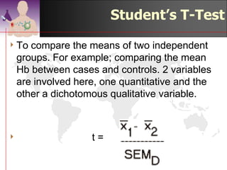
Student's T-test, Paired T-Test, ANOVA & Proportionate Test
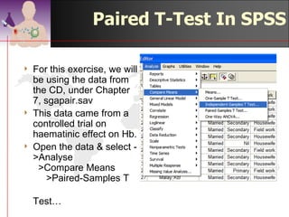
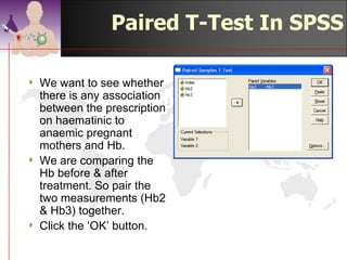
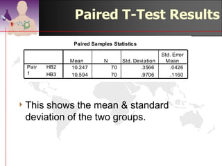
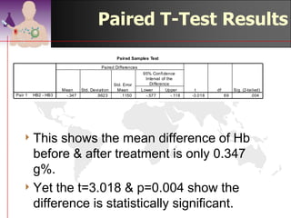
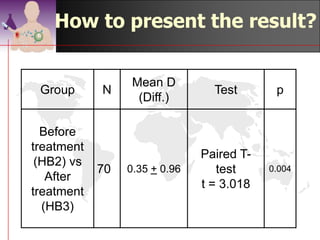
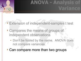
This document discusses various statistical tests including the T-test, ANOVA, and proportionate tests. It provides details on the independent T-test, paired T-test, ANOVA, and examples of using each test. Key concepts covered include the Student's T-test, its assumptions, and how to perform manual calculations and analyze data using SPSS.
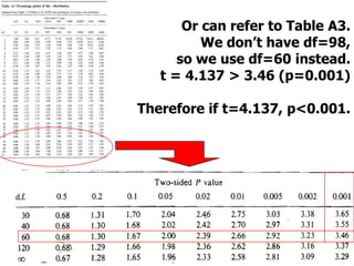
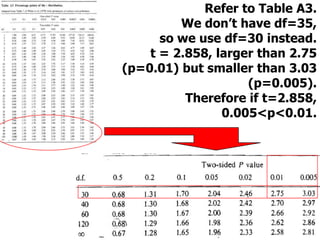
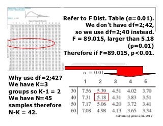
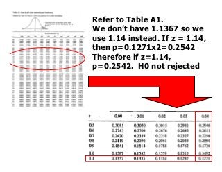
Refer to TableA3.
We don’t have df=35,
so we use df=30 instead.
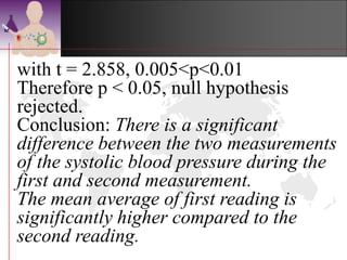
t = 2.858, larger than 2.75
(p=0.01) but smaller than 3.03
(p=0.005). 3.03>t>2.75
Therefore if t=2.858,
0.005<p<0.01.
24.93
Example:
Time To Complete
Analysis
45samples were
analysed using 3 different
blood analyser (Mach1,
Mach2 & Mach3).
22.61
15 samples were placed
into each analyser.
Time in seconds was
measured for each 20.59
sample analysis.
44.
24.93
Example:
Time To Complete
Analysis
Theoverall mean of the
entire sample was 22.71
seconds. 22.71
22.61
This is called the “grand”
mean, and is often
denoted by X .
If H0 were true then we’d
expect the group means 20.59
to be close to the grand
mean.
45.
24.93
Example:
Time To Complete
Analysis
TheANOVA test is
based on the combined
distances from X .
22.71
If the combined 22.61
distances are large, that
indicates we should
reject H0.
20.59
46.
The Anova Statistic
Tocombine the differences from the grand mean we
• Square the differences
• Multiply by the numbers of observations in the groups
• Sum over the groups
( )2
( )
2
(
SSB = 15 X Mach1 − X + 15 X Mach 2 − X + 15 X Mach3 − X )
2
where the X * are the group means.
“SSB” = Sum of Squares Between groups
47.
The Anova Statistic
Tocombine the differences from the grand mean we
• Square the differences
• Multiply by the numbers of observations in the groups
• Sum over the groups
( )2
( )
2
(
SSB = 15 X Mach1 − X + 15 X Mach 2 − X + 15 X Mach3 − X )
2
where the X * are the group means.
“SSB” = Sum of Squares Between groups
Note: This looks a bit like a variance.
How big isbig?
4 For the Time to Complete, SSB = 141.492
4 Is that big enough to reject H0?
4 As with the t test, we compare the statistic to
the variability of the individual observations.
4 InANOVA the variability is estimated by the
Mean Square Error, or MSE
50.
MSE
Mean Square Error
The Mean Square Error
is a measure of the
variability after the
group effects have
been taken into
account.
∑∑ (x − X j)
1 2
MSE = ij
N −K j i
where xij is the ith
observation in the jth
group.
51.
MSE
Mean Square Error
24.93
The Mean Square Error
is a measure of the
variability after the
group effects have
been taken into
22.61
account.
∑∑ (x − X j)
1 2
MSE = ij
N −K j i
20.59
where xij is the ith
observation in the jth
group.
52.
MSE
Mean Square Error
24.93
The Mean Square Error
is a measure of the
variability after the
group effects have
been taken into
22.61
account.
∑∑ (x − X j)
1 2
MSE = ij
N −K j i
20.59
Notes on MSE
4Ifthere are only two groups, the MSE is equal
to the pooled estimate of variance used in the
equal-variance t test.
4 ANOVA assumes that all the group variances
are equal.
4 Other options should be considered if group
variances differ by a factor of 2 or more.
4 (12.8380 ~ 9.4160 ~ 11.1262)
56.
ANOVA F Test
4The ANOVA F test is based on the F statistic
SSB (K − 1)
F=
MSE
where K is the number of groups.
4 Under H0 the F statistic has an “F” distribution,
with K-1 and N-K degrees of freedom (N is the
total number of observations)
57.
Time to Analyse:
F test p-value
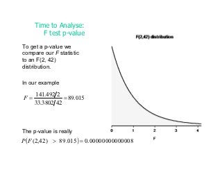
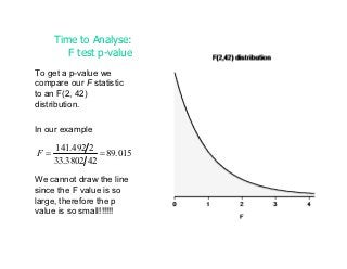
To get a p-value we
compare our F statistic
to an F(2, 42)
distribution.
58.
Time to Analyse:
F test p-value
To get a p-value we
compare our F statistic
to an F(2, 42)
distribution.
In our example
141.492 2
F= = 89.015
33.3802 42
We cannot draw the line
since the F value is so
large, therefore the p
value is so small!!!!!!
Time to Analyse:
F test p-value
To get a p-value we
compare our F statistic
to an F(2, 42)
distribution.
In our example
141.492 2
F= = 89.015
33.3802 42
The p-value is really
P(F (2,42) > 89.015) = 0.00000000000008
61.
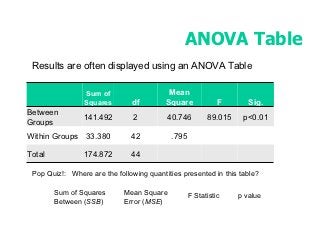
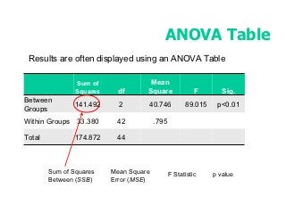
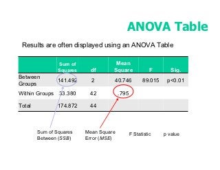
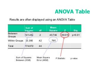
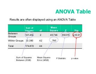
ANOVA Table
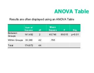
Resultsare often displayed using an ANOVA Table
Sum of Mean
Squares df Square F Sig.
Between
141.492 2 40.746 89.015 p<0.01
Groups
Within Groups 33.380 42 .795
Total 174.872 44
62.
ANOVA Table
Resultsare often displayed using an ANOVA Table
Sum of Mean
Squares df Square F Sig.
Between
141.492 2 40.746 89.015 p<0.01
Groups
Within Groups 33.380 42 .795
Total 174.872 44
Pop Quiz!: Where are the following quantities presented in this table?
Sum of Squares Mean Square F Statistic p value
Between (SSB) Error (MSE)
63.
ANOVA Table
Resultsare often displayed using an ANOVA Table
Sum of Mean
Squares df Square F Sig.
Between
141.492 2 40.746 89.015 p<0.01
Groups
Within Groups 33.380 42 .795
Total 174.872 44
Sum of Squares Mean Square F Statistic p value
Between (SSB) Error (MSE)
64.
ANOVA Table
Resultsare often displayed using an ANOVA Table
Sum of Mean
Squares df Square F Sig.
Between
141.492 2 40.746 89.015 p<0.01
Groups
Within Groups 33.380 42 .795
Total 174.872 44
Sum of Squares Mean Square F Statistic p value
Between (SSB) Error (MSE)
65.
ANOVA Table
Resultsare often displayed using an ANOVA Table
Sum of Mean
Squares df Square F Sig.
Between
141.492 2 40.746 89.015 p<0.01
Groups
Within Groups 33.380 42 .795
Total 174.872 44
Sum of Squares Mean Square F Statistic p value
Between (SSB) Error (MSE)
66.
ANOVA Table
Resultsare often displayed using an ANOVA Table
Sum of Mean
Squares df Square F Sig.
Between
141.492 2 40.746 89.015 p<0.01
Groups
Within Groups 33.380 42 .795
Total 174.872 44
Sum of Squares Mean Square F Statistic p value
Between (SSB) Error (MSE)
#39 79 Note: There is one dependent variable in the ANOVA model. MANOVA has more than one dependent variable. Ask, what are nominal & interval scales?