Downloaded 268 times

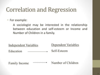
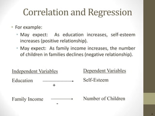
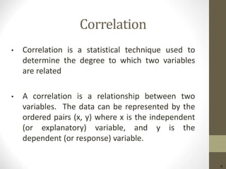
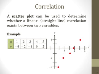
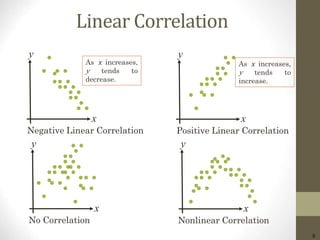
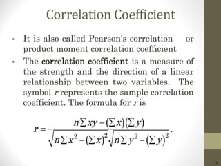
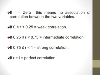
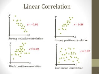
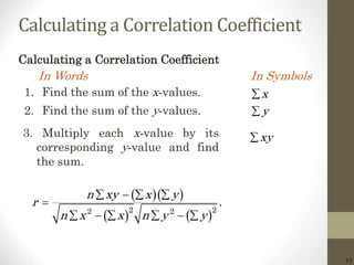
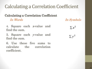
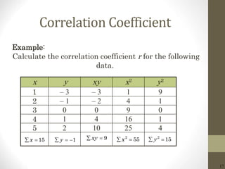
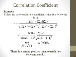
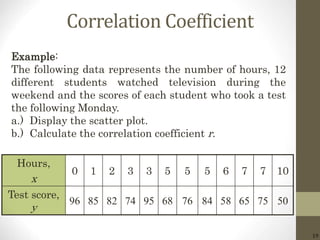
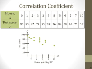
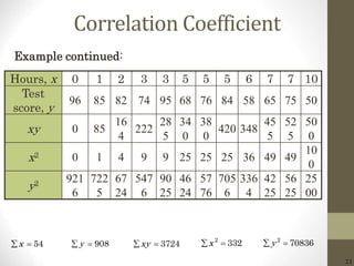
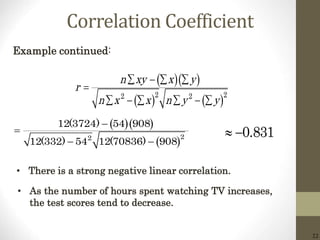
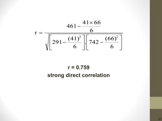
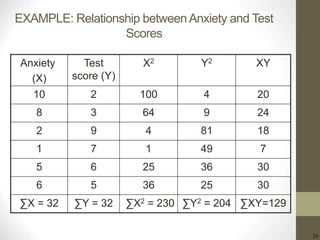
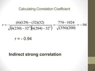
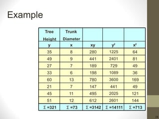
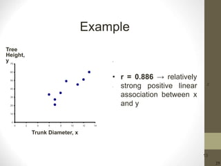
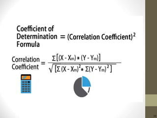
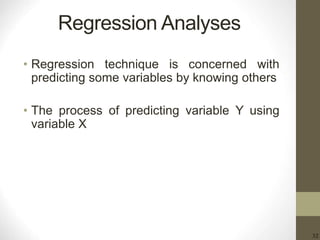
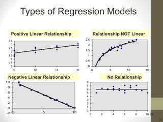
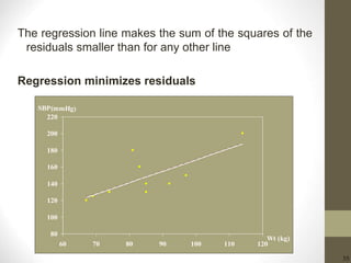
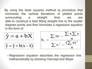
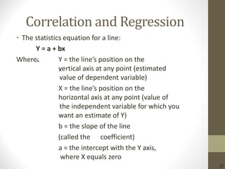
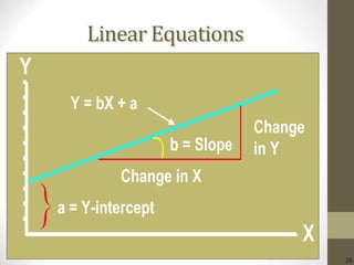
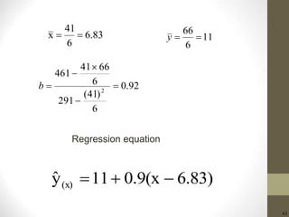
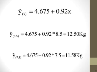
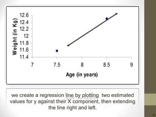
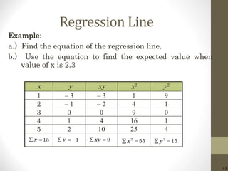
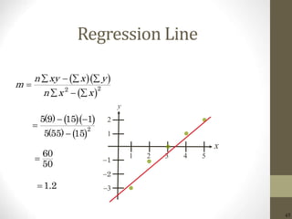
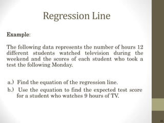
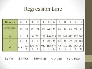
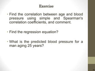
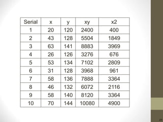
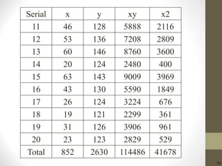
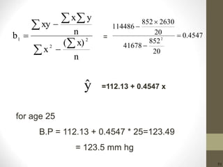

This document discusses correlation and regression. Correlation describes the strength and direction of a linear relationship between two variables, while regression allows predicting a dependent variable from an independent variable. It provides examples of calculating the correlation coefficient r to determine the strength and direction of relationships between variables like education and self-esteem or family income and number of children. The regression equation describes the linear regression line and can be used to predict values of the dependent variable from known values of the independent variable.


![[Deck] What's New in Spark-Iceberg Integration via DSV2.pptx](https://cdn.slidesharecdn.com/ss_thumbnails/deckwhatsnewinspark-icebergintegrationviadsv2-260210005337-25955b12-thumbnail.jpg?width=640&height=640&fit=bounds)

