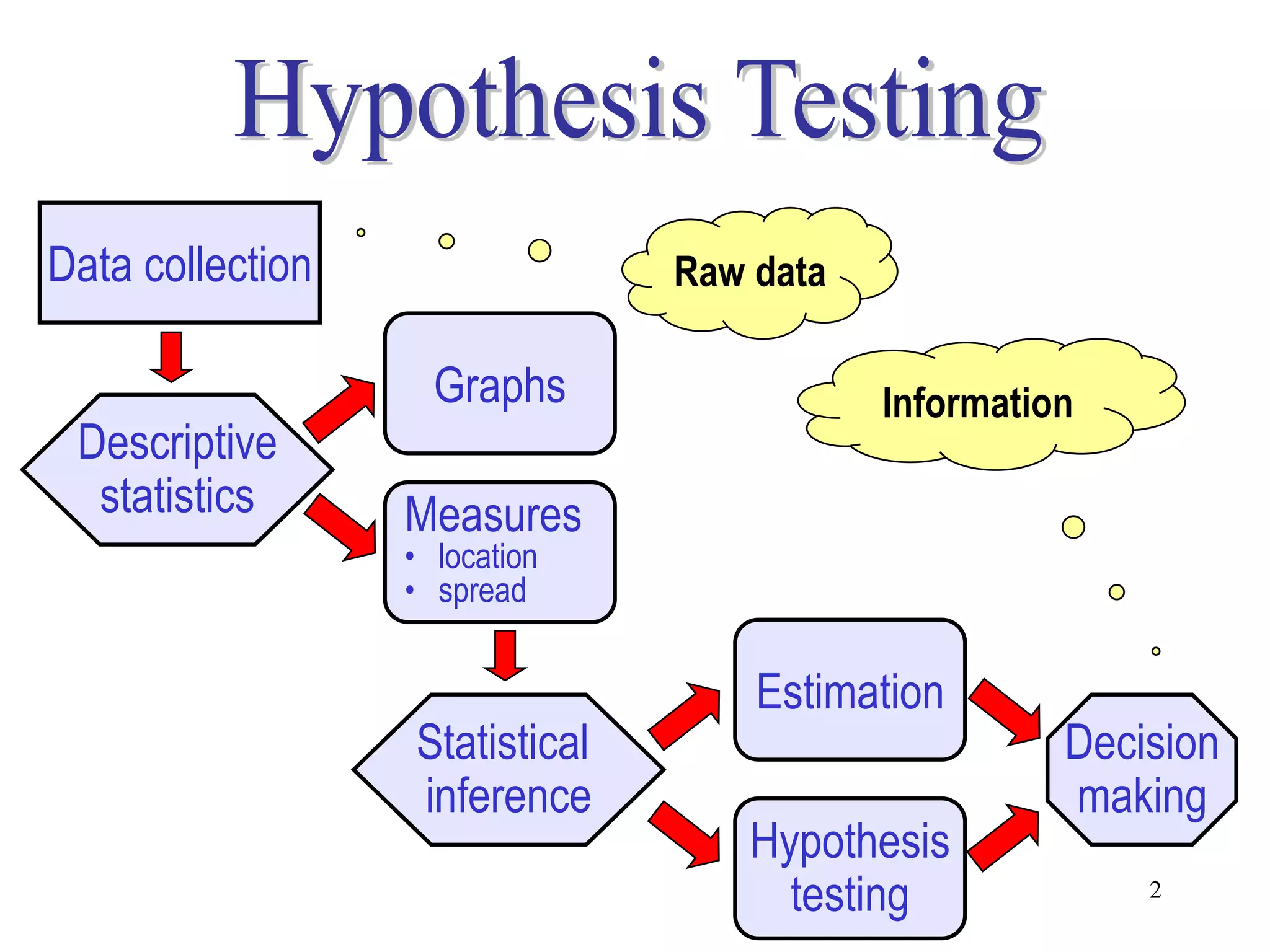
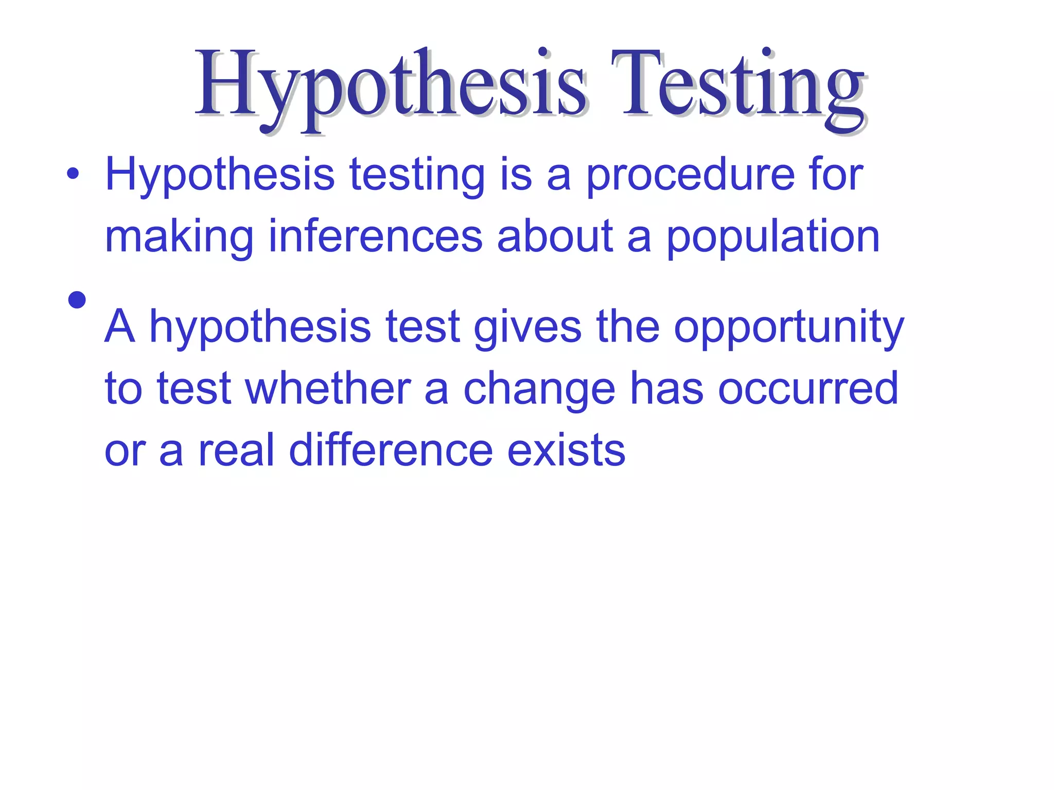
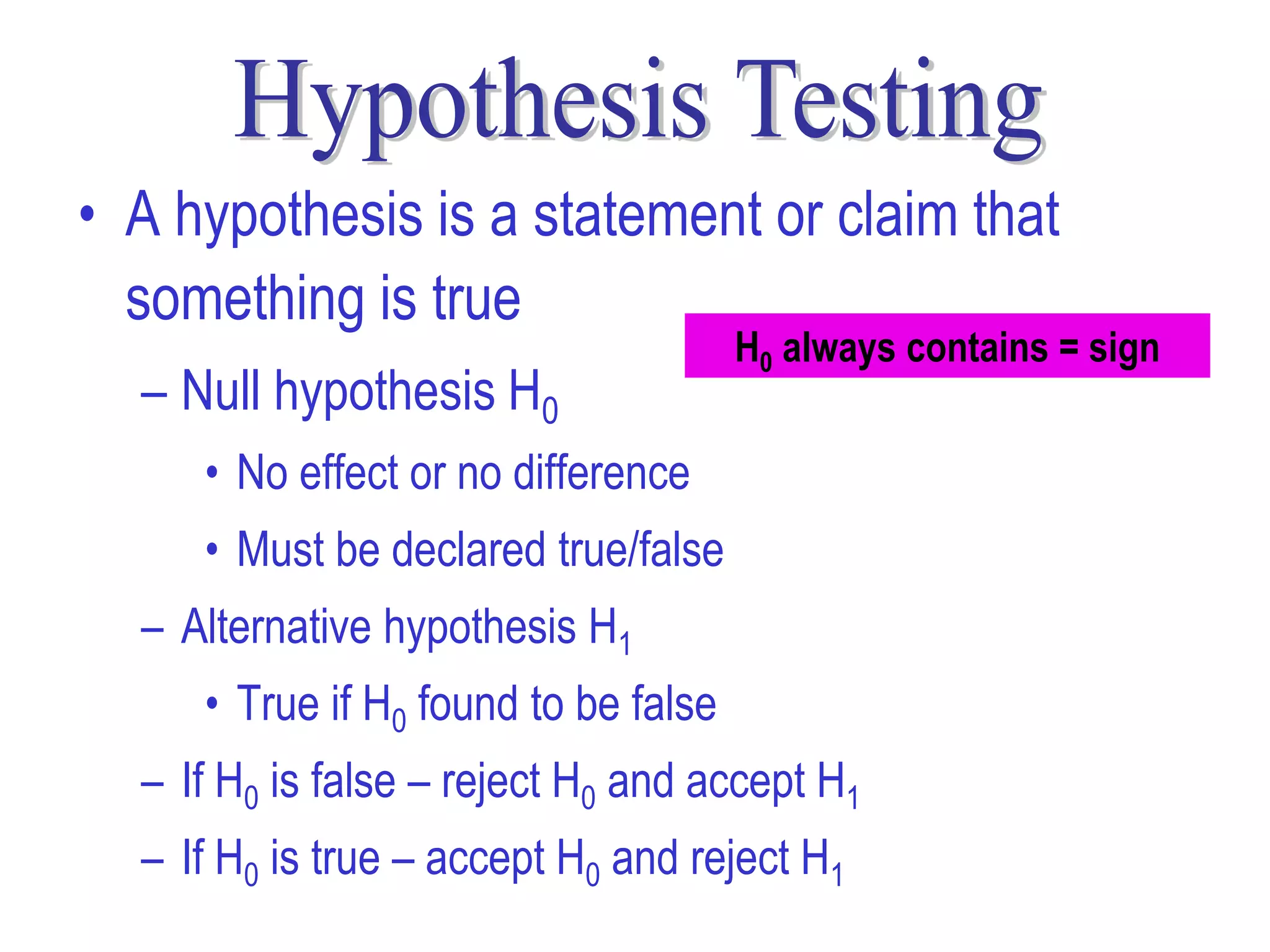
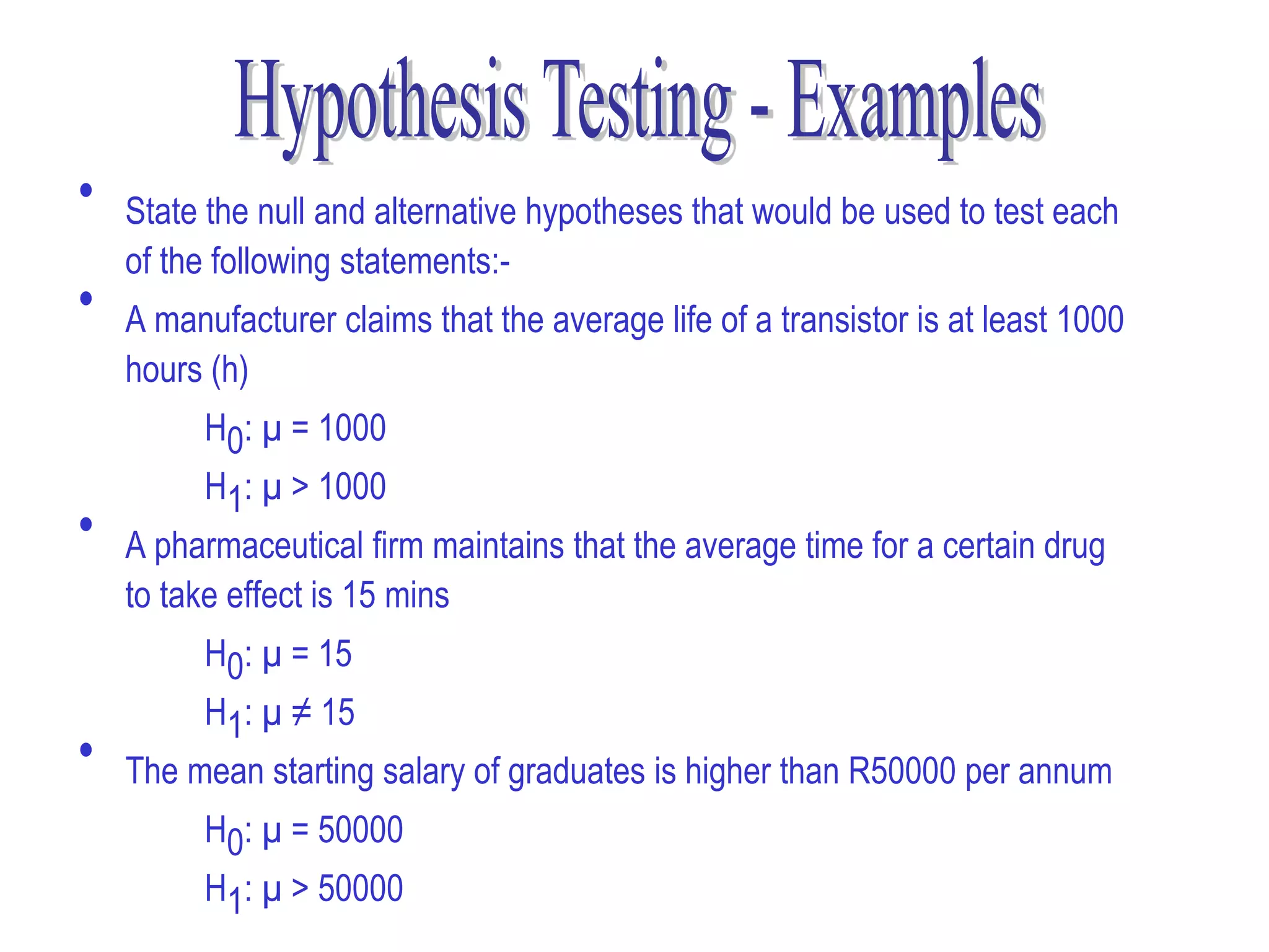
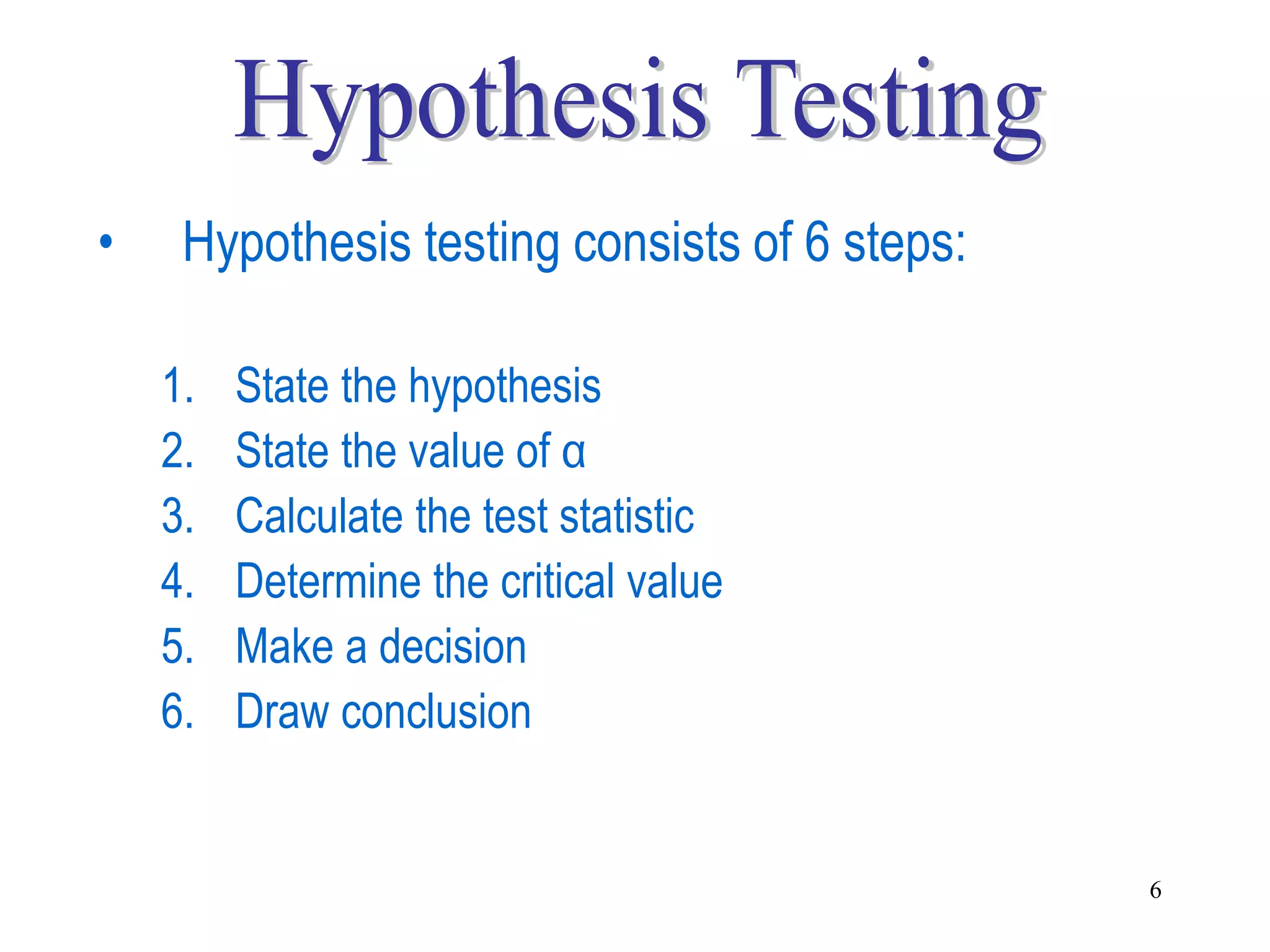
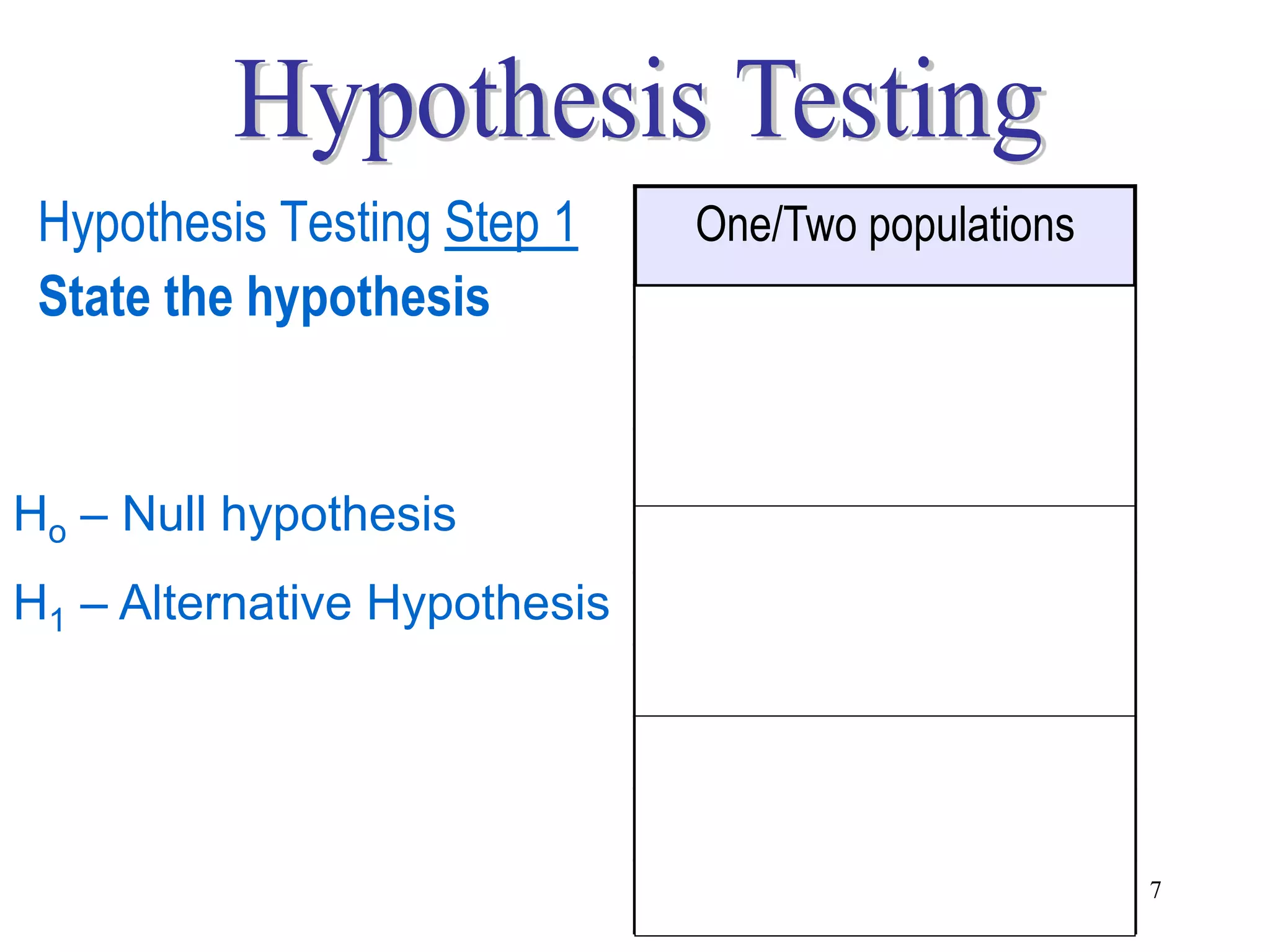
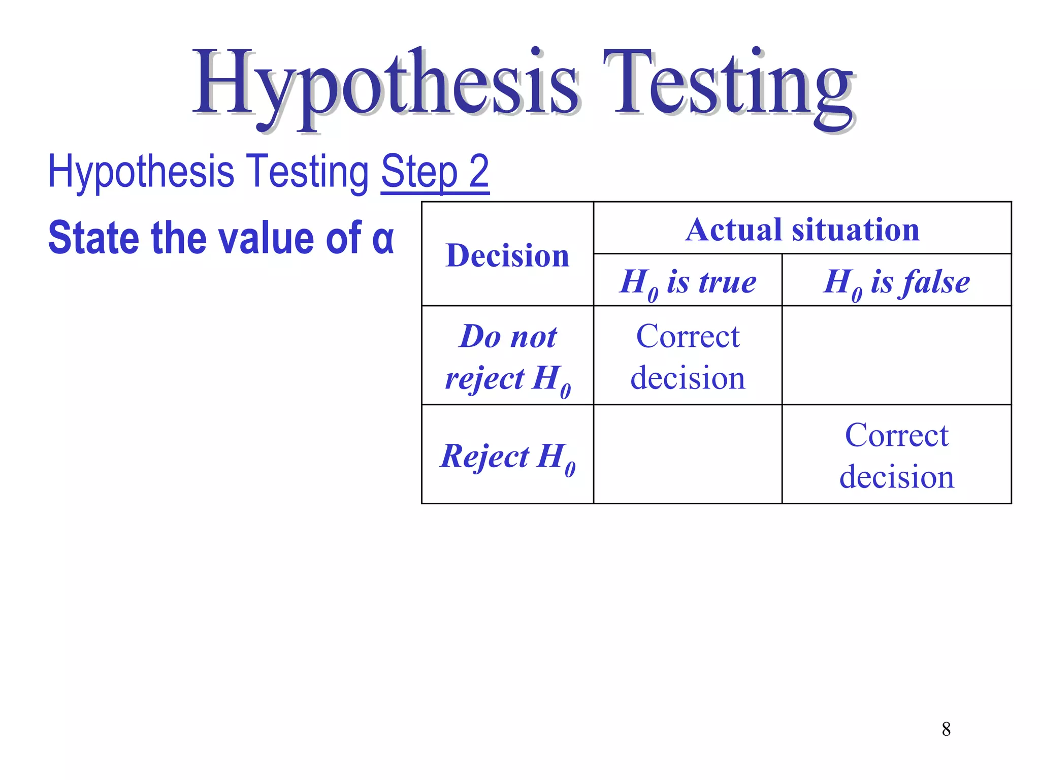
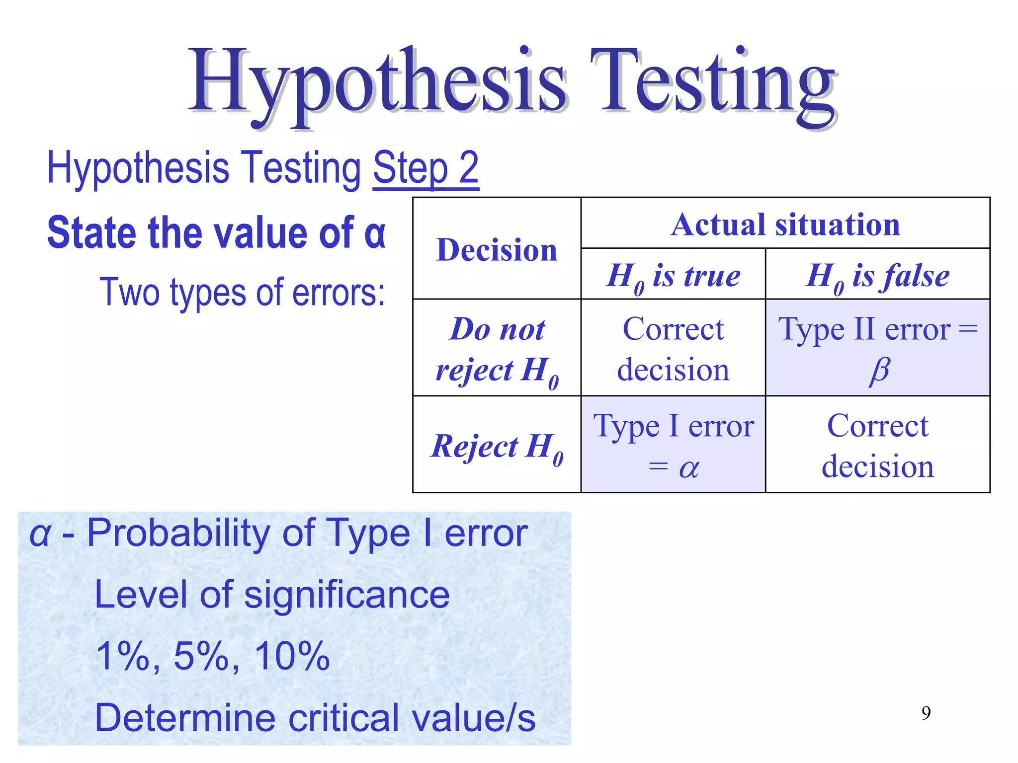
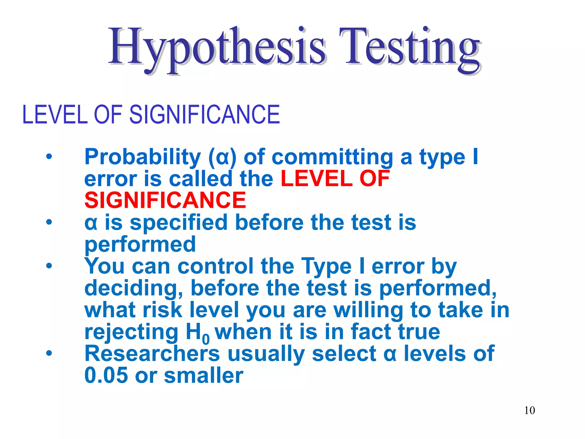
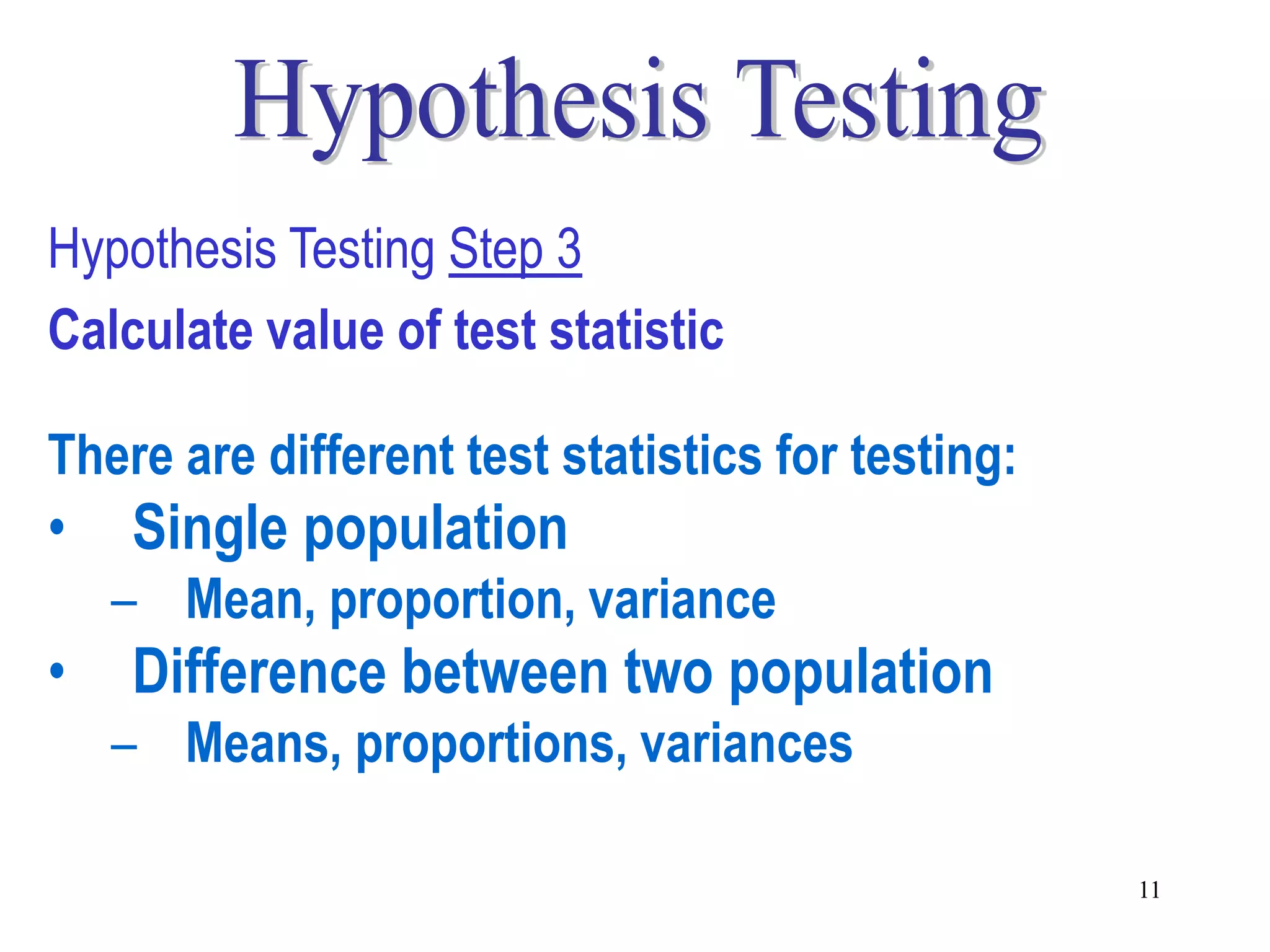
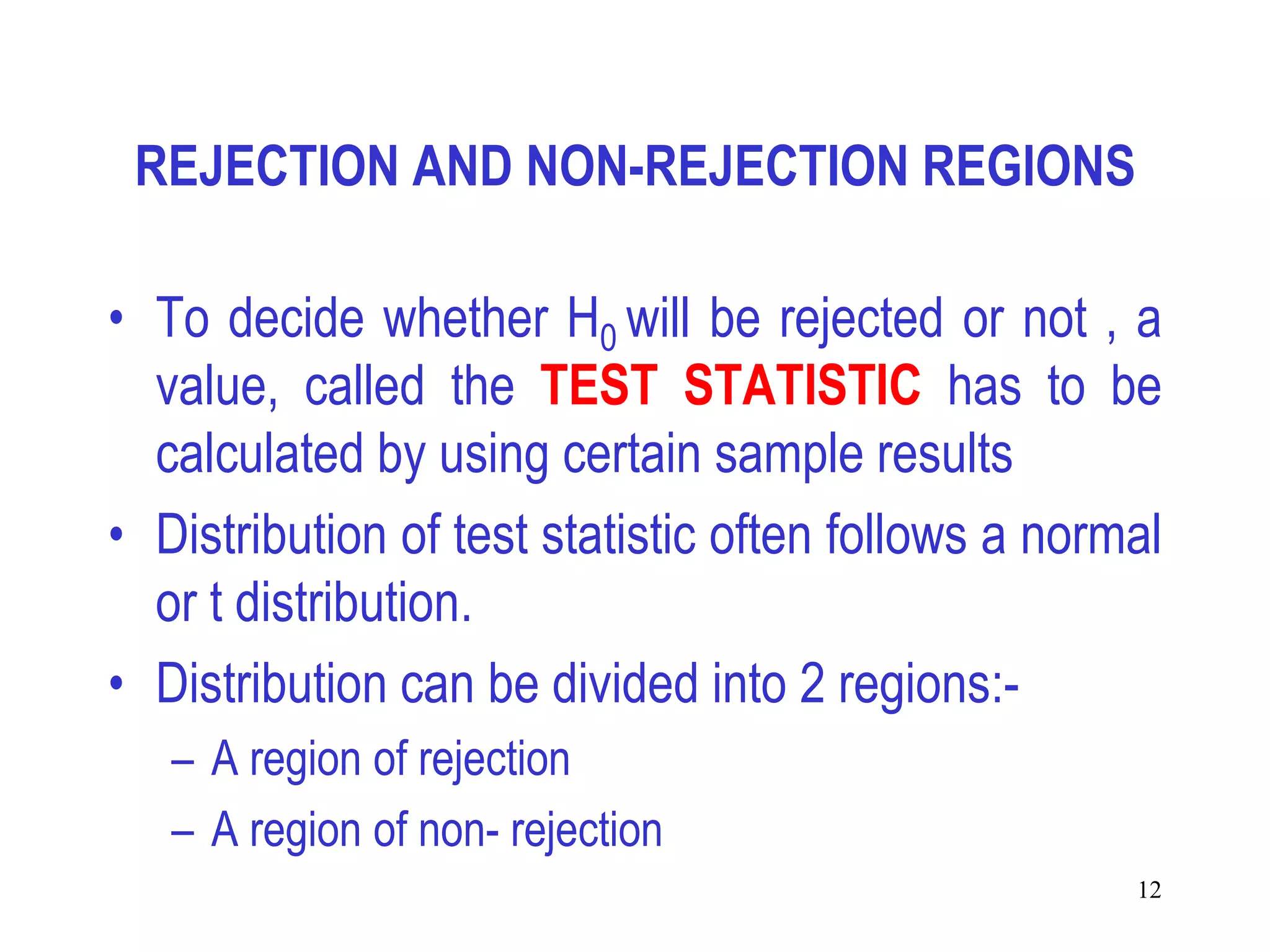
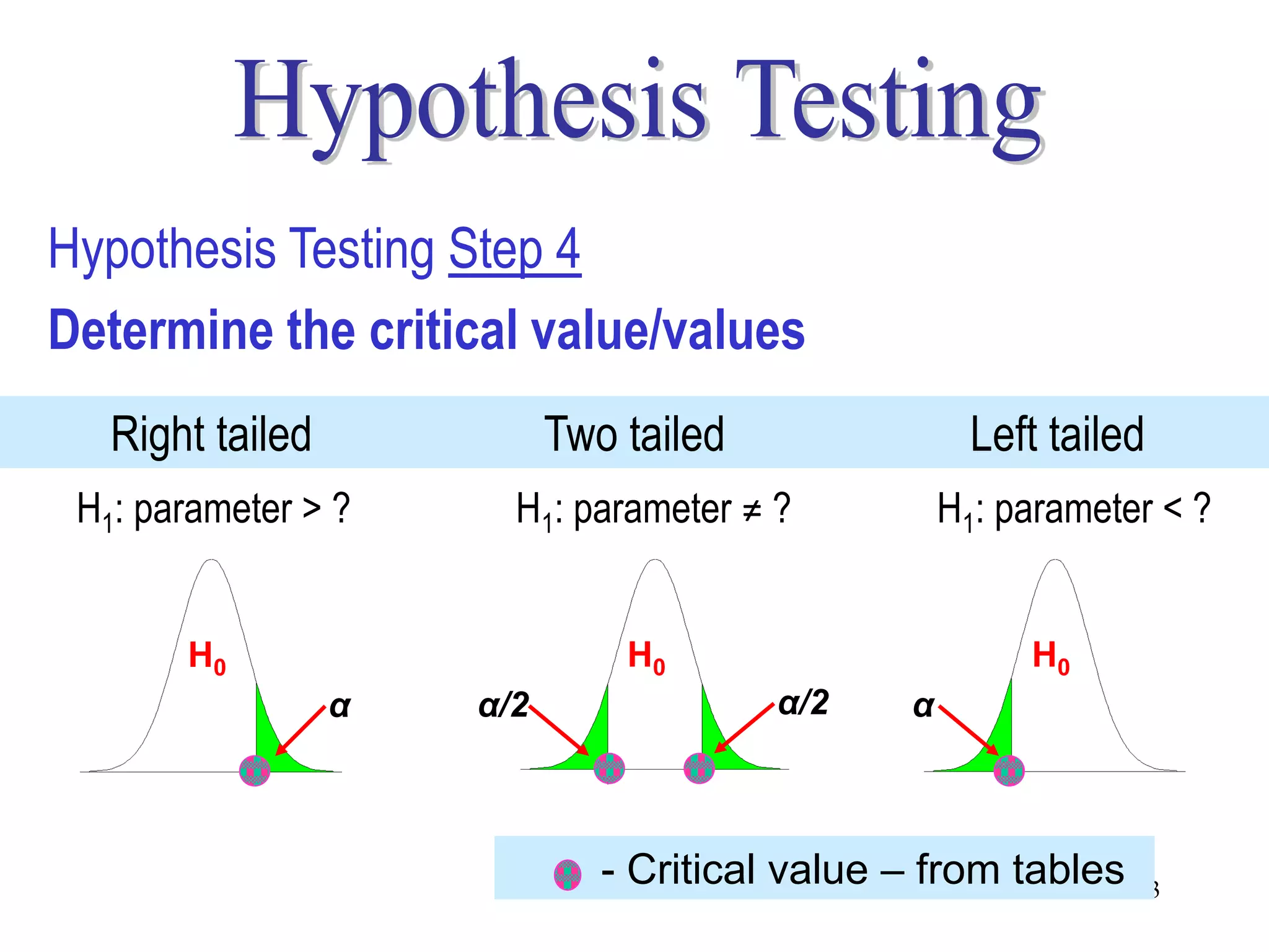
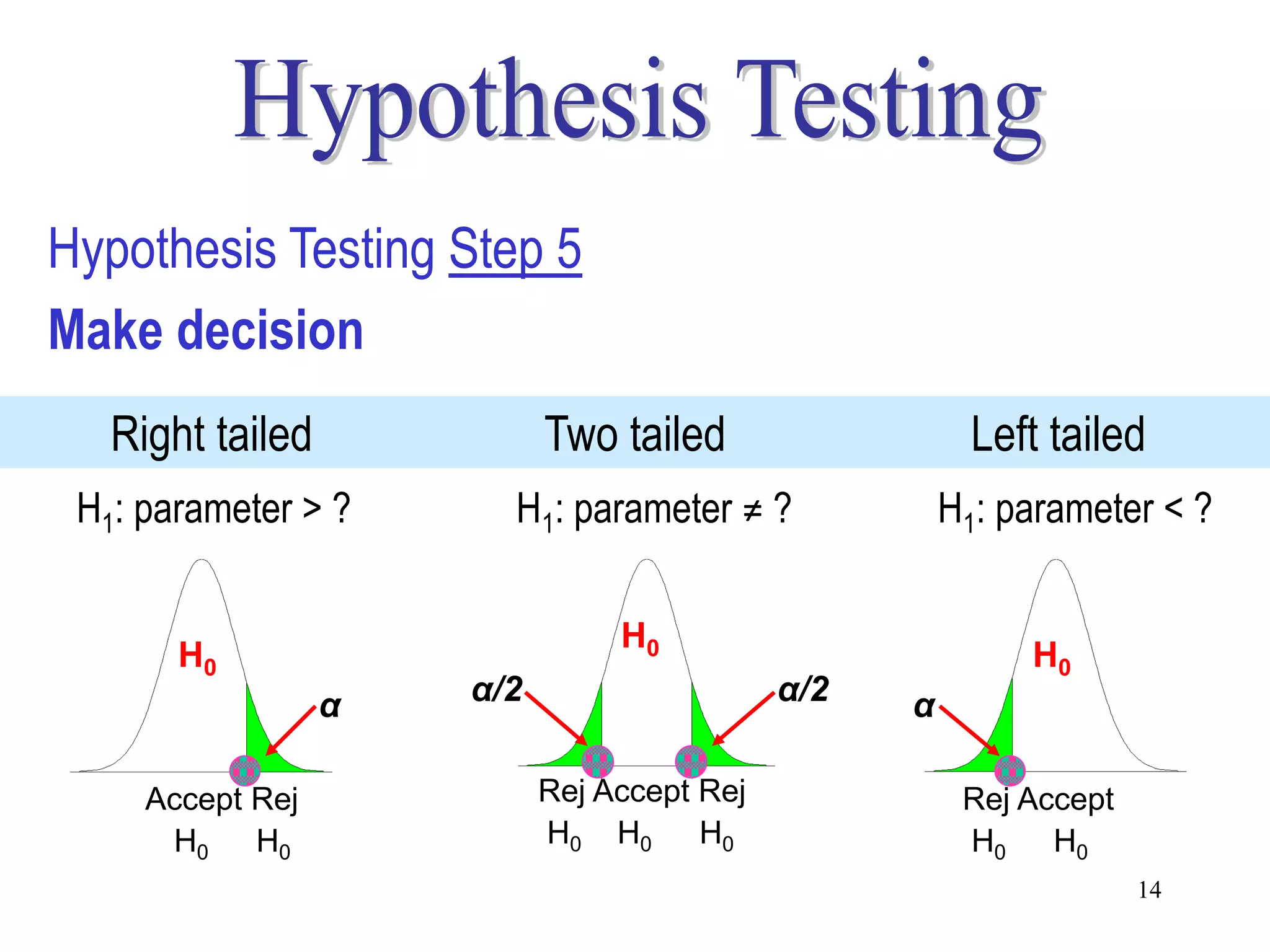
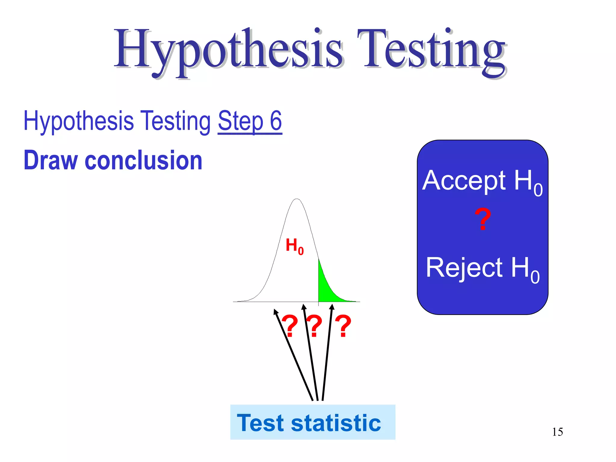
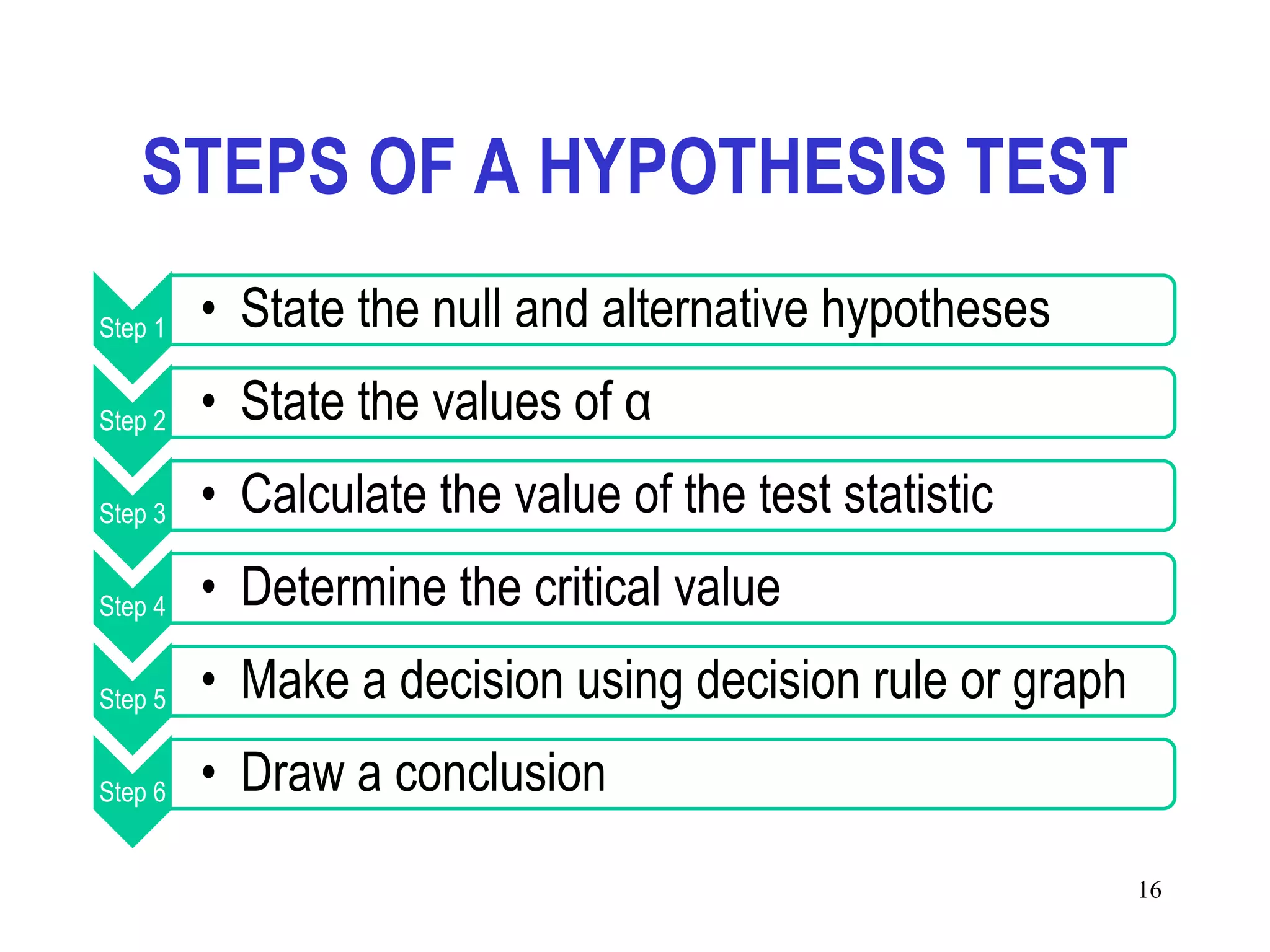
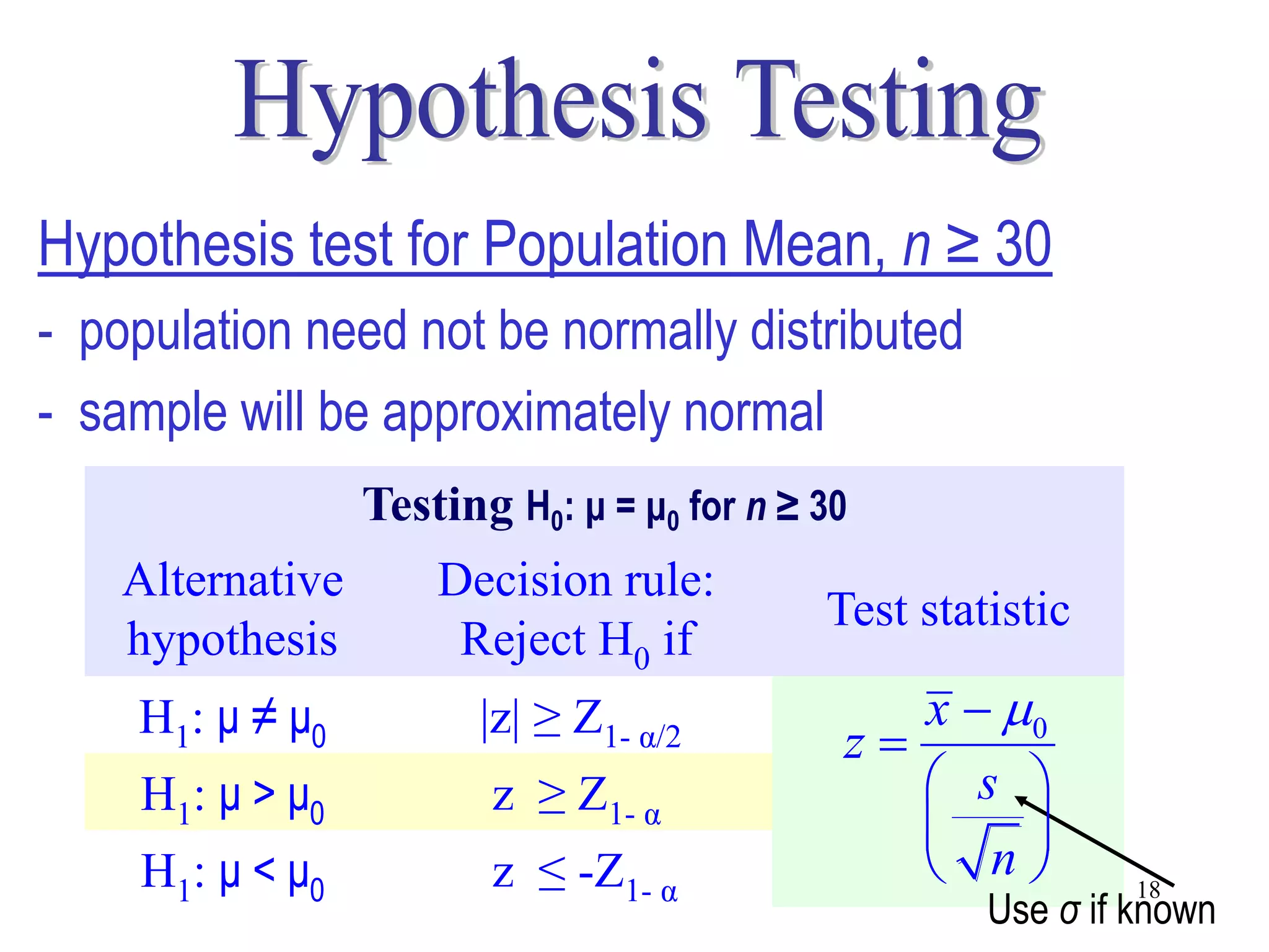
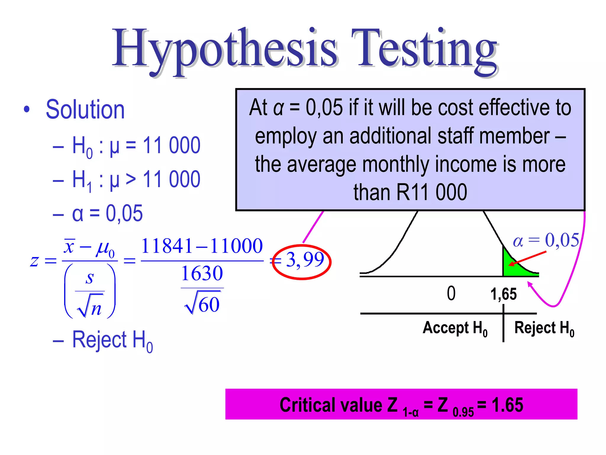
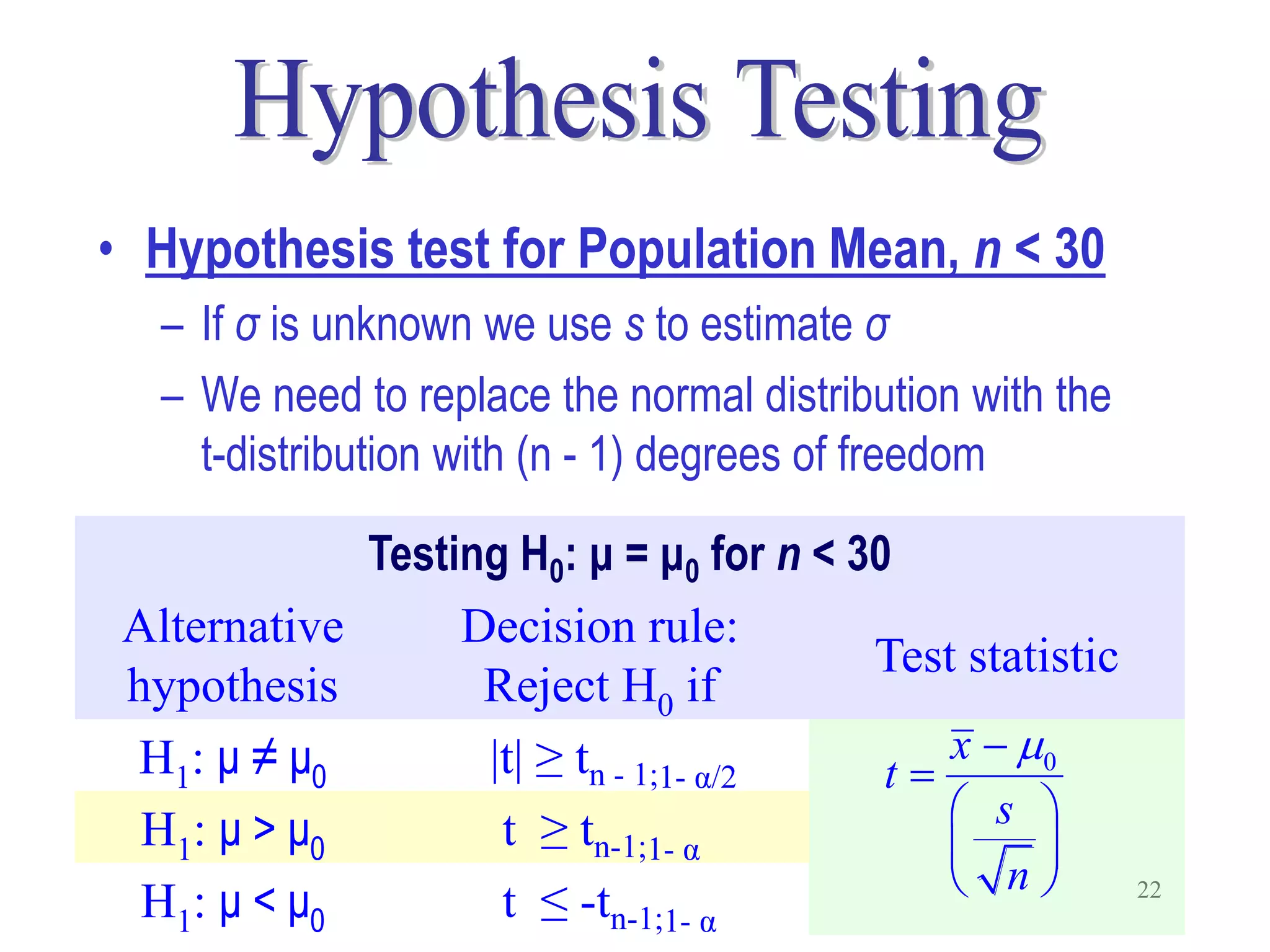
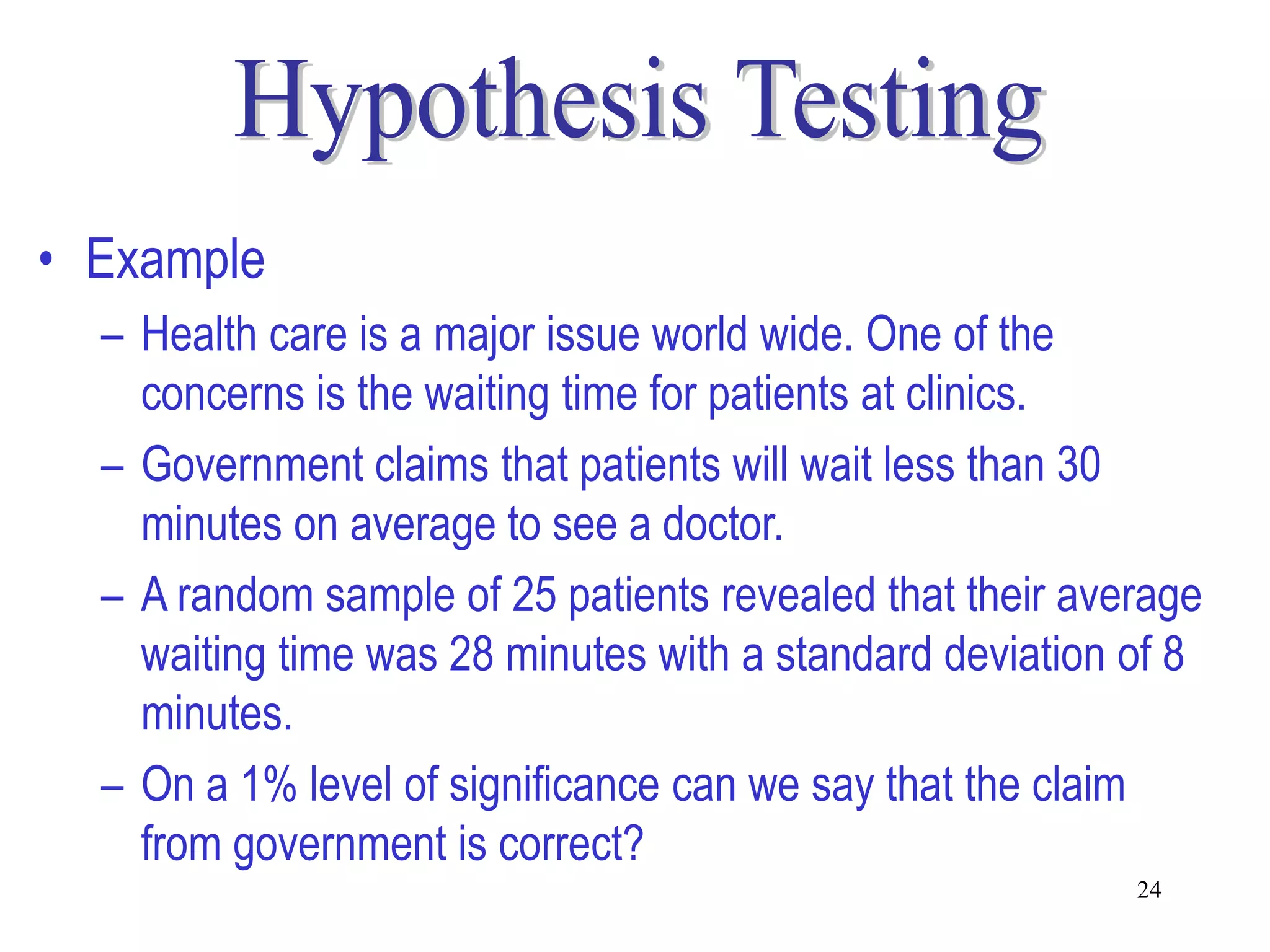
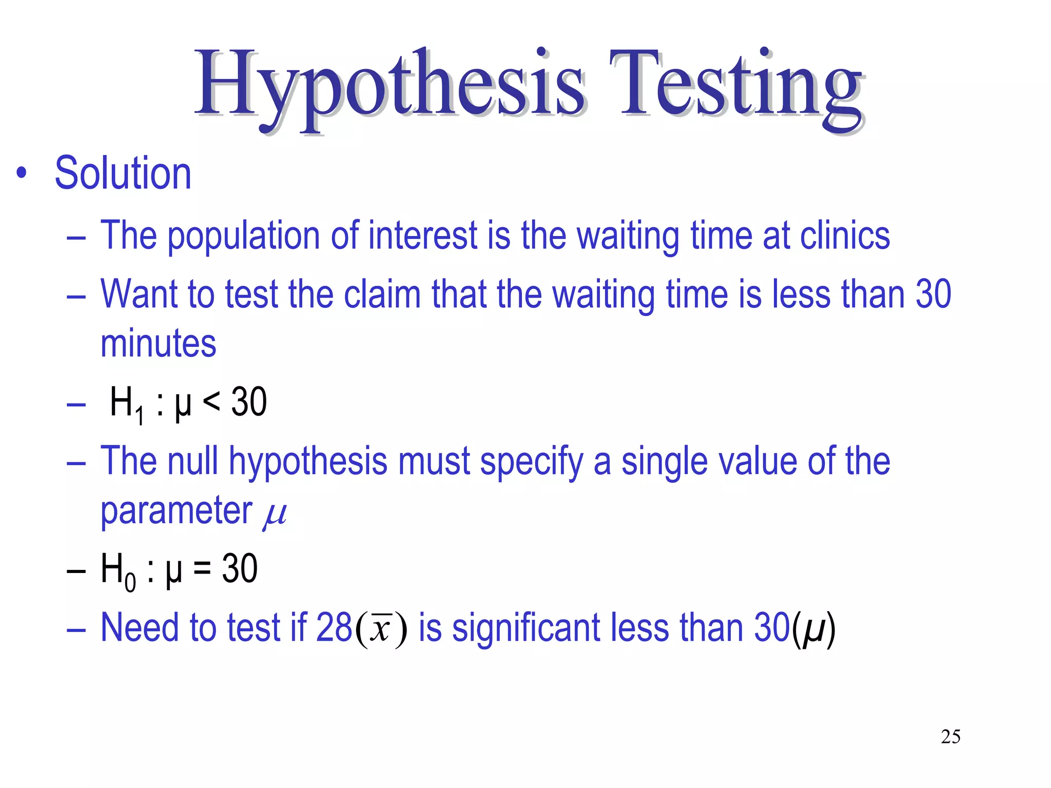
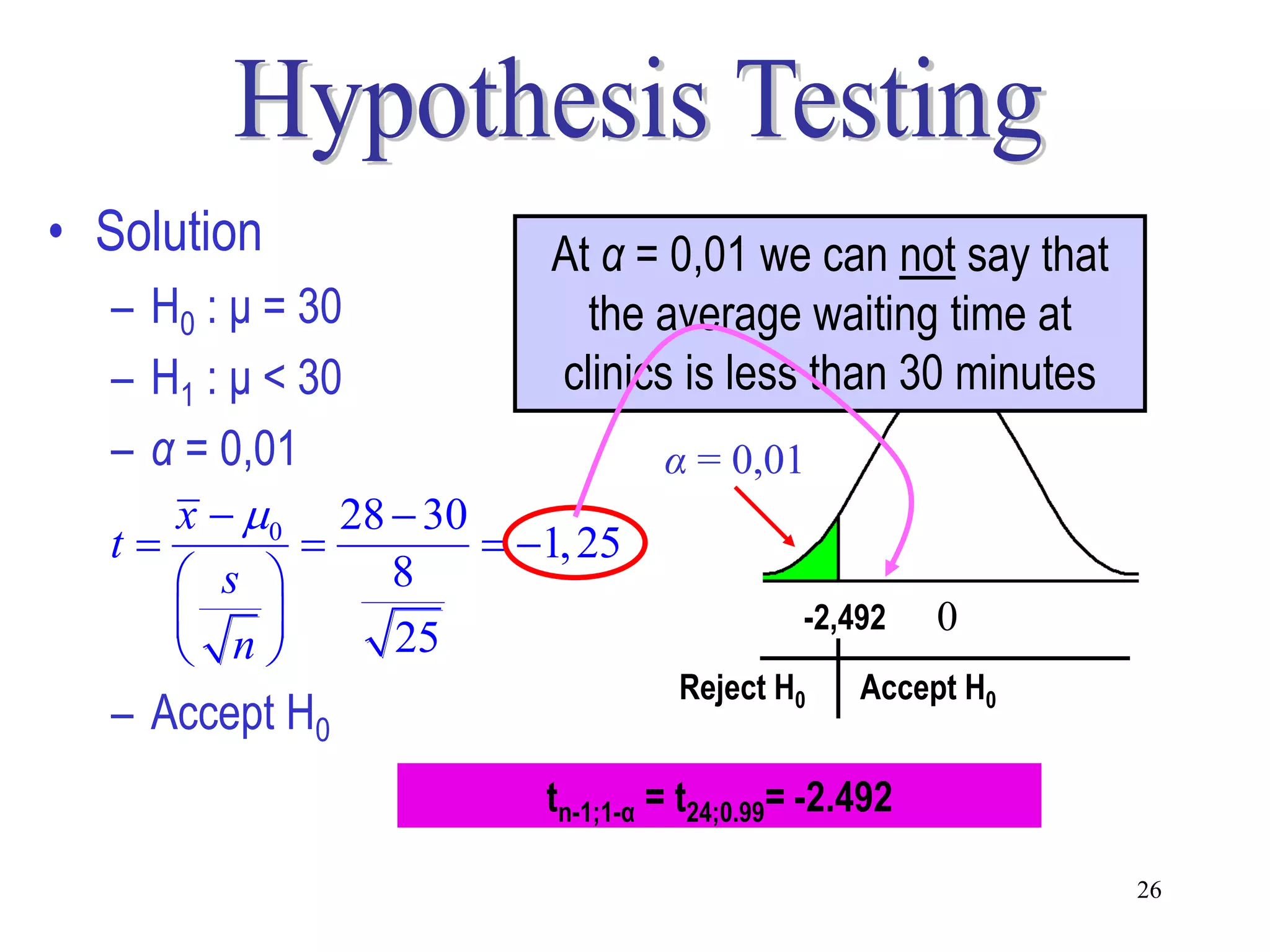
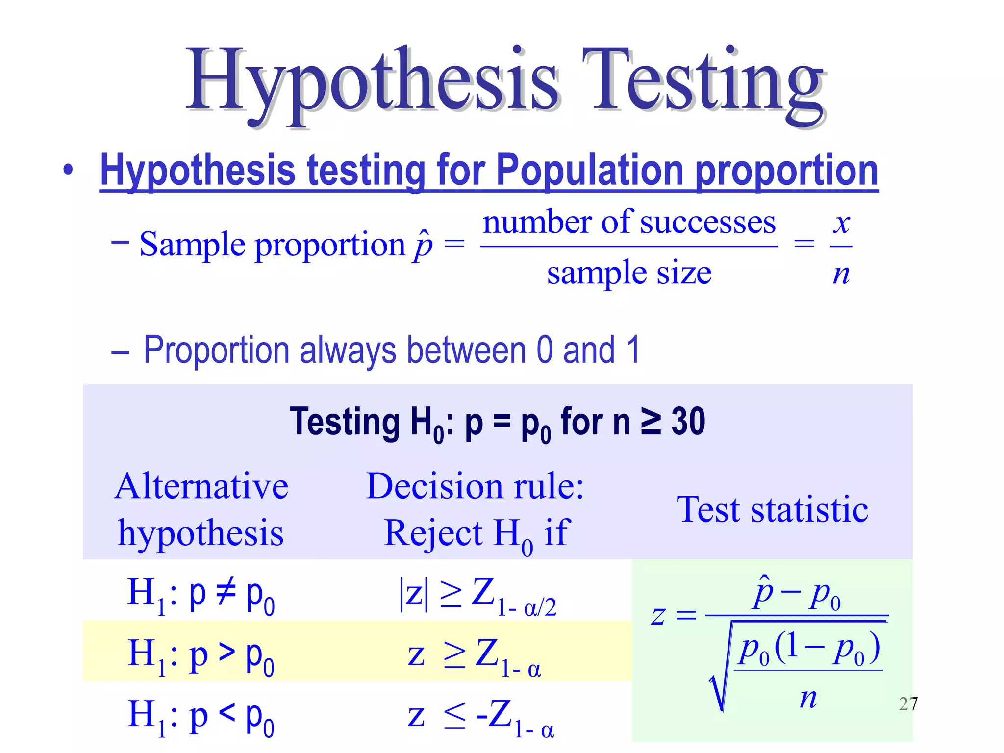
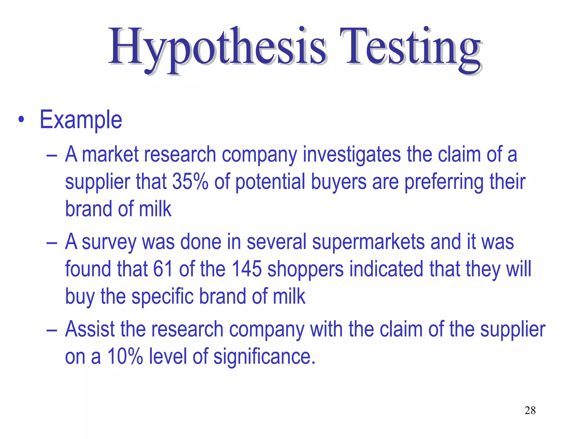
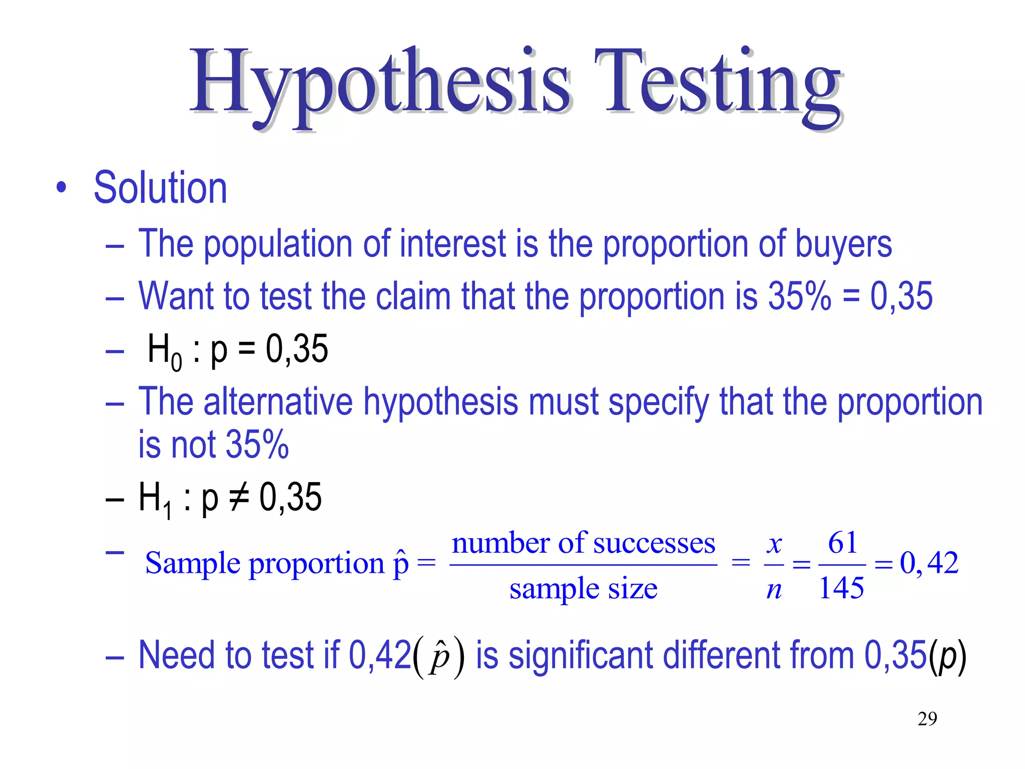
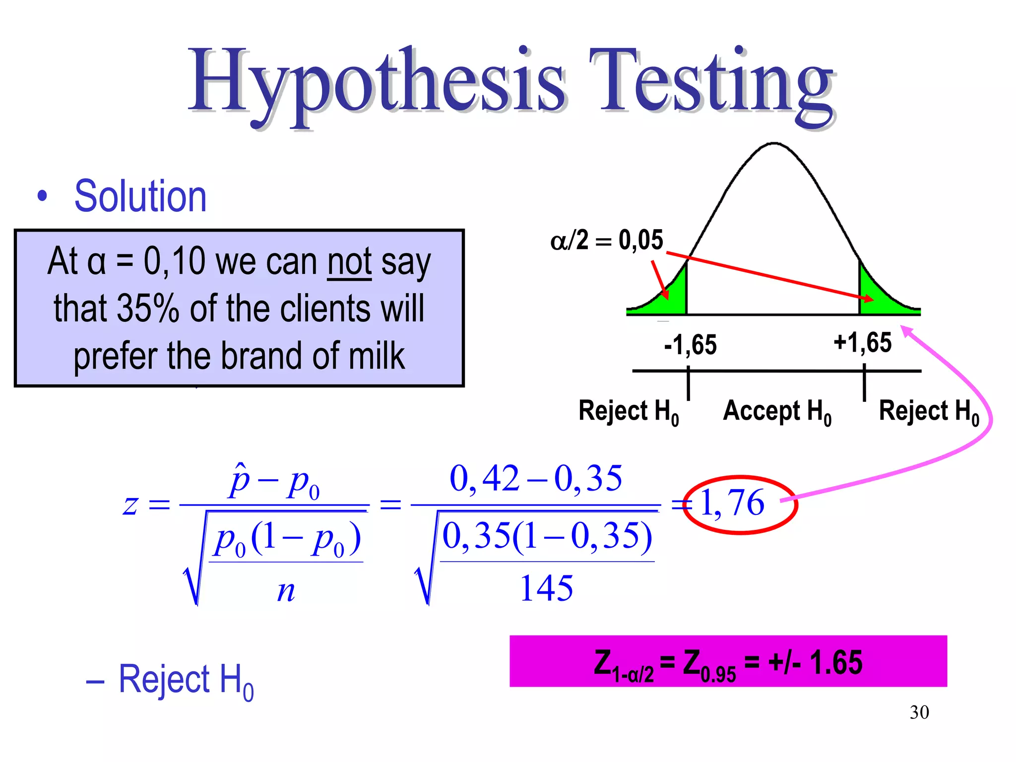
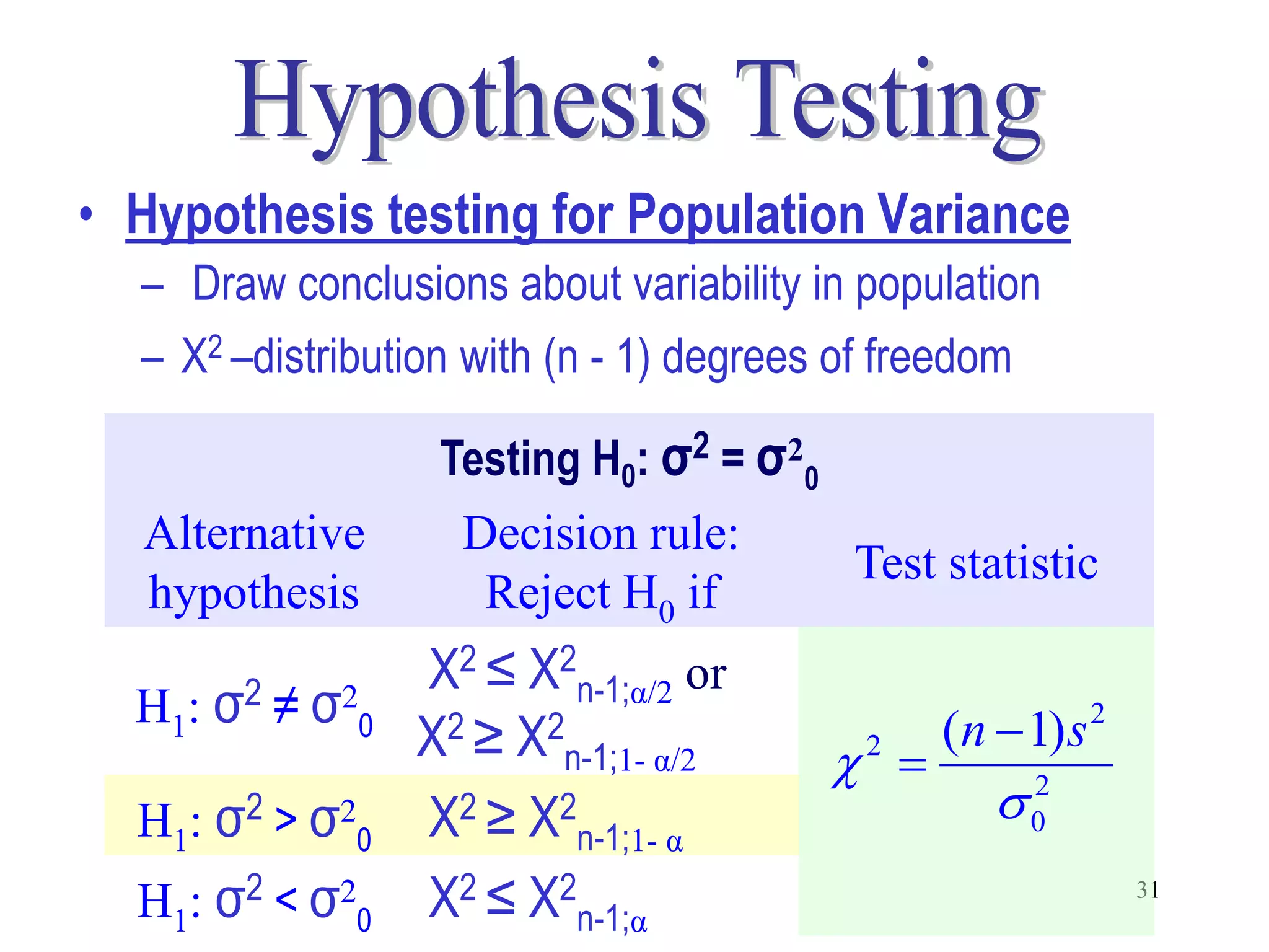
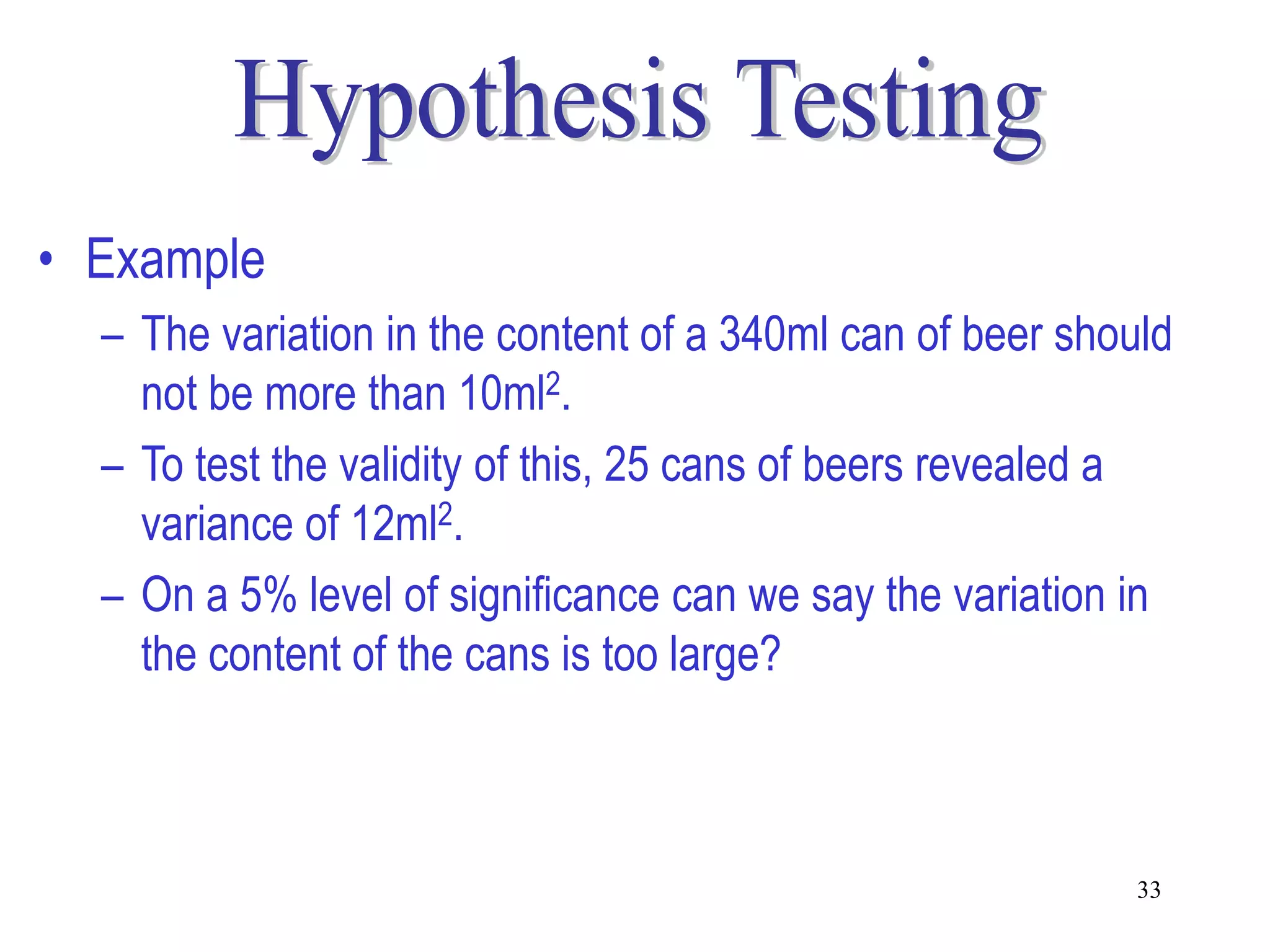
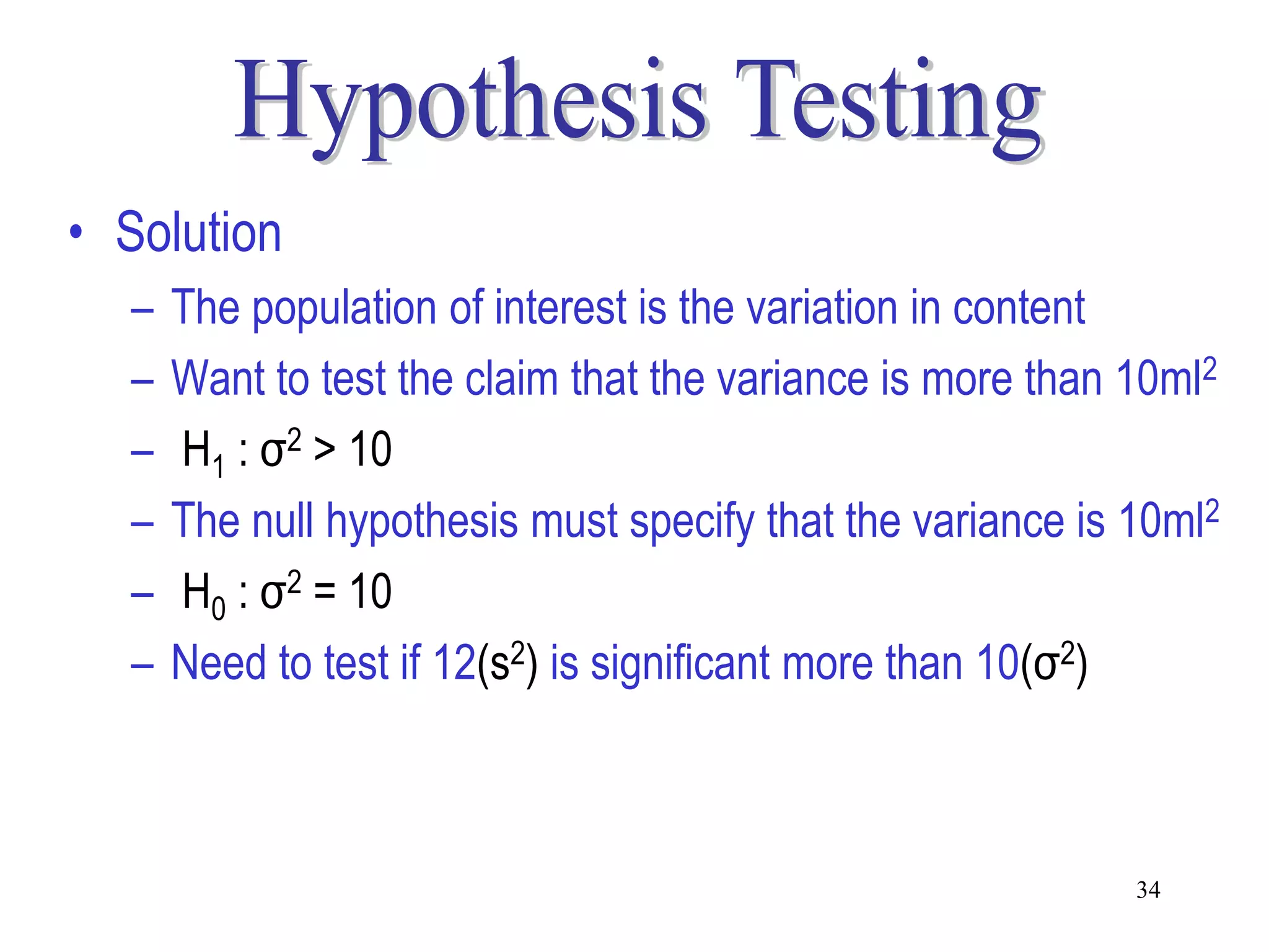
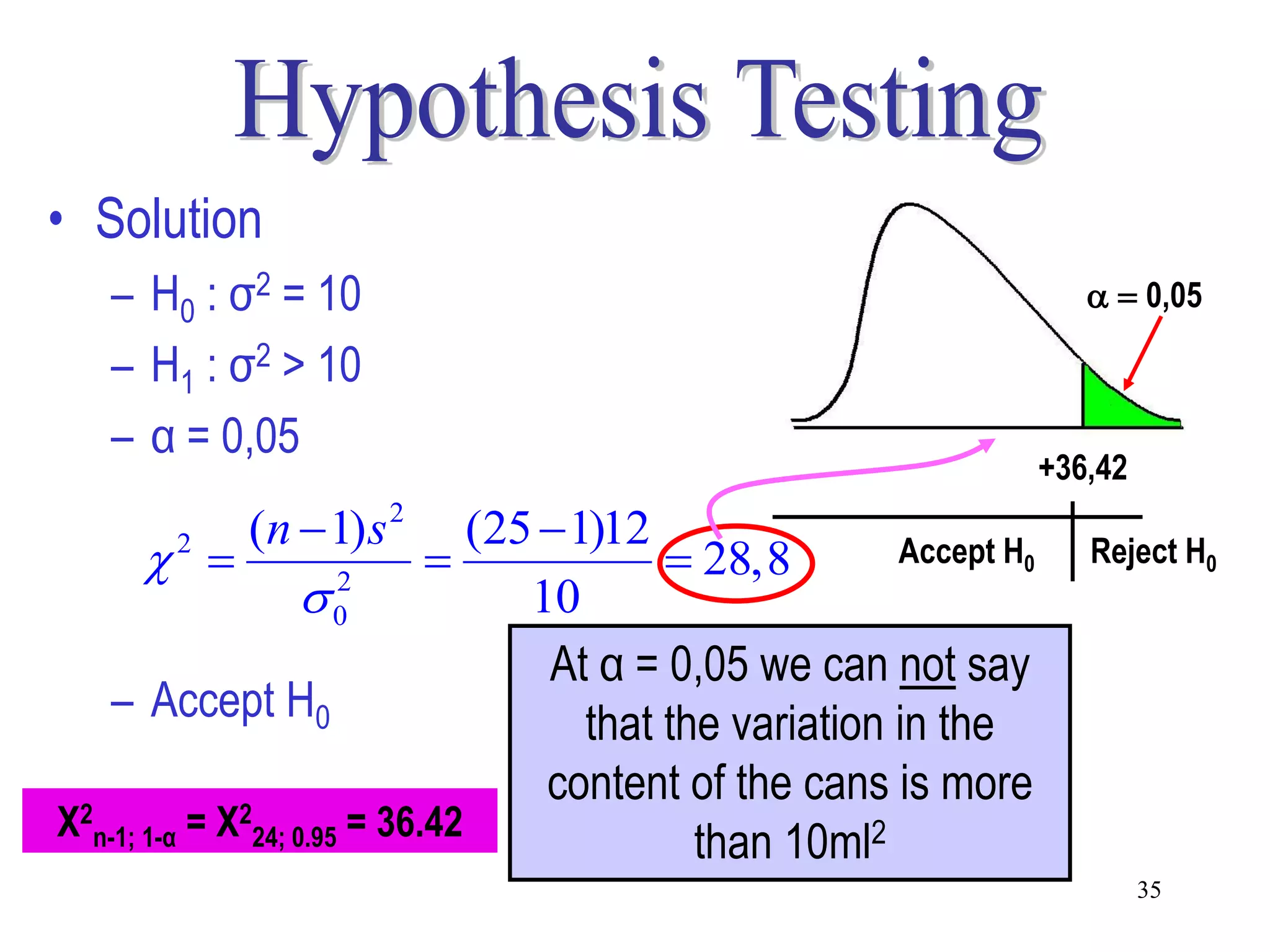
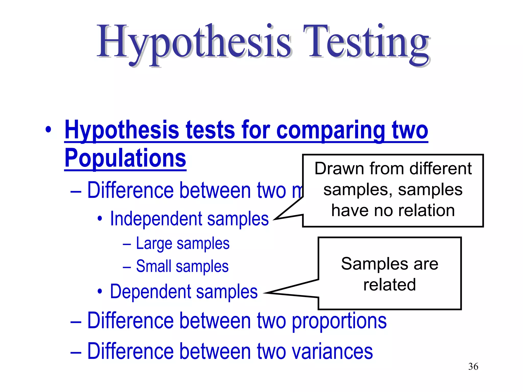
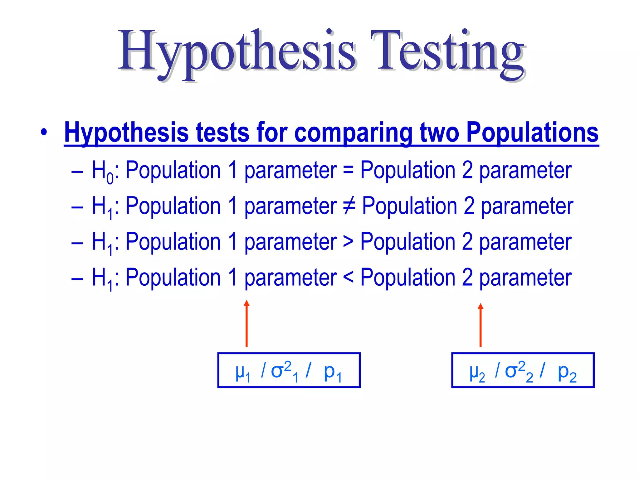
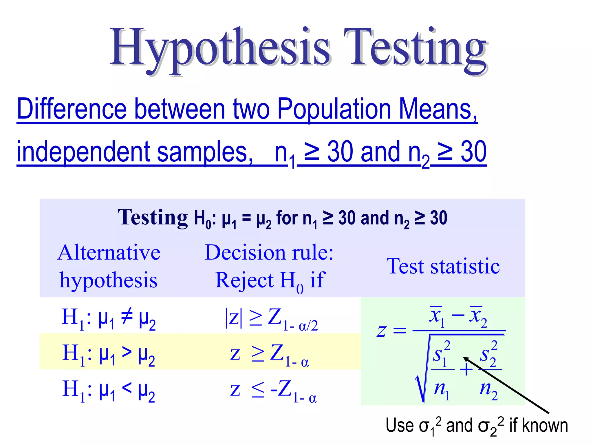
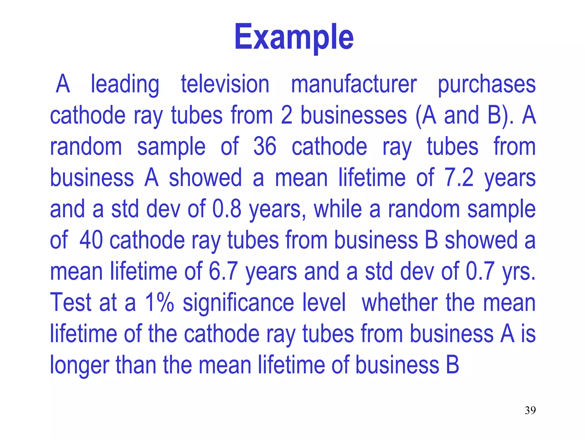
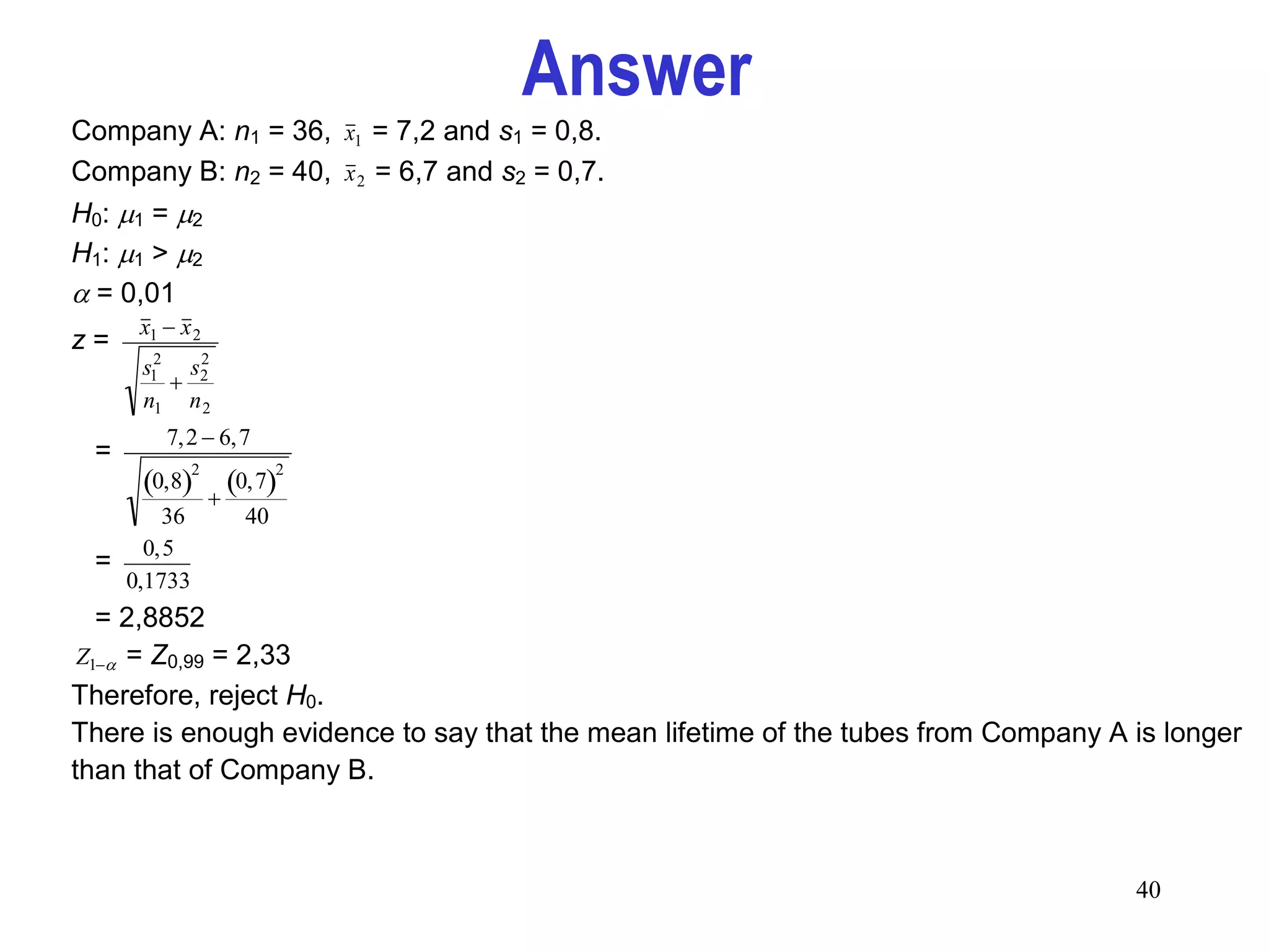
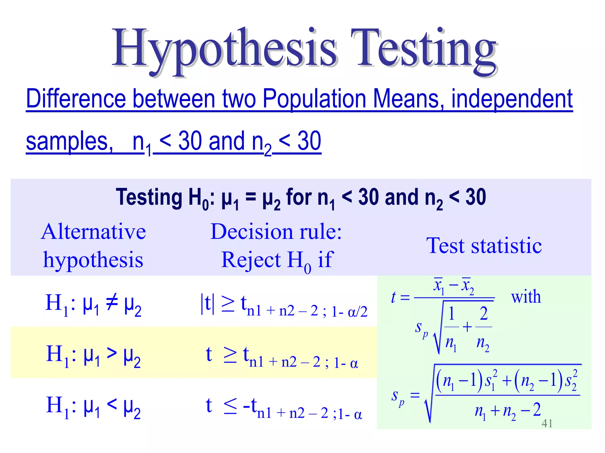
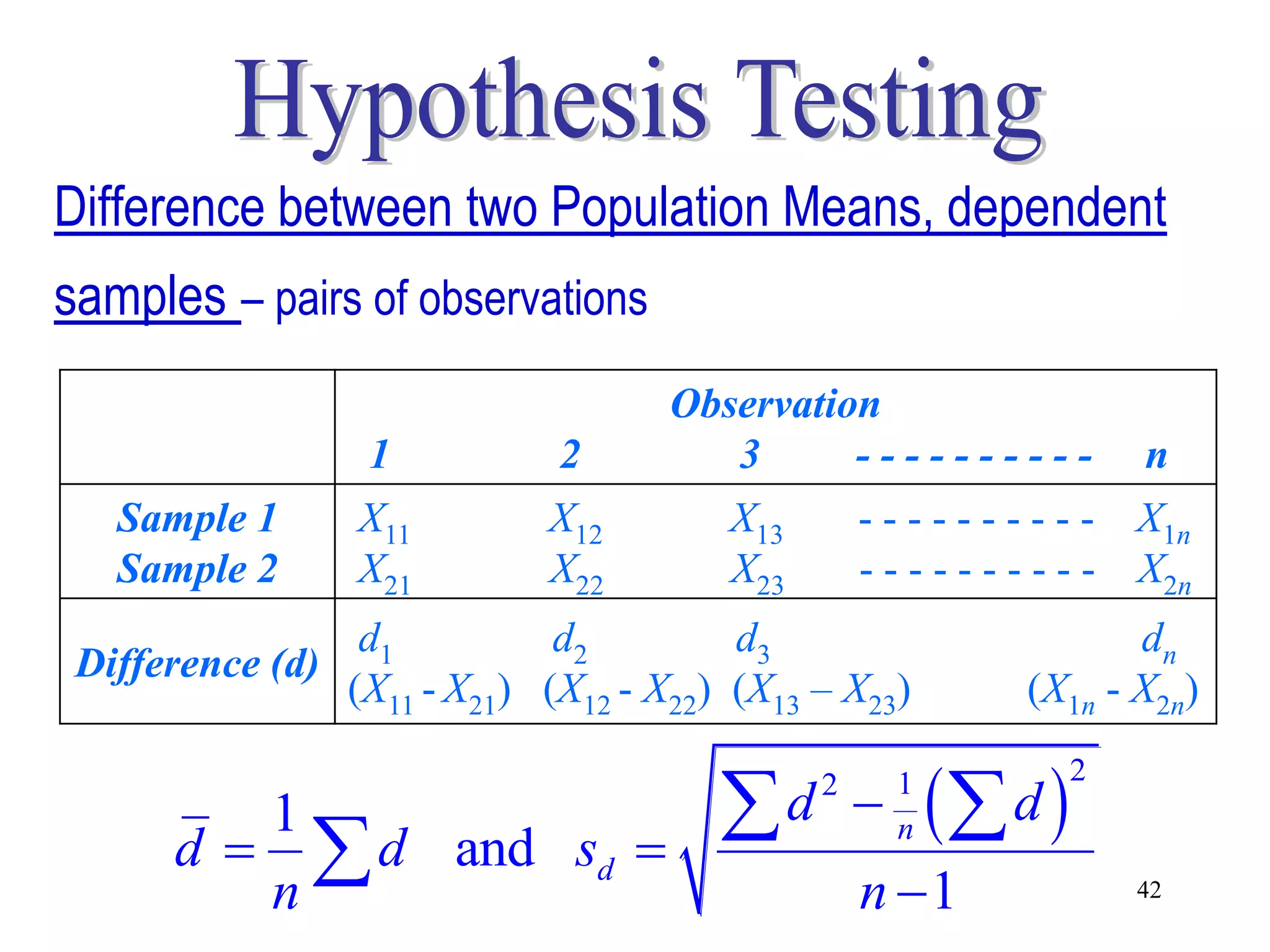
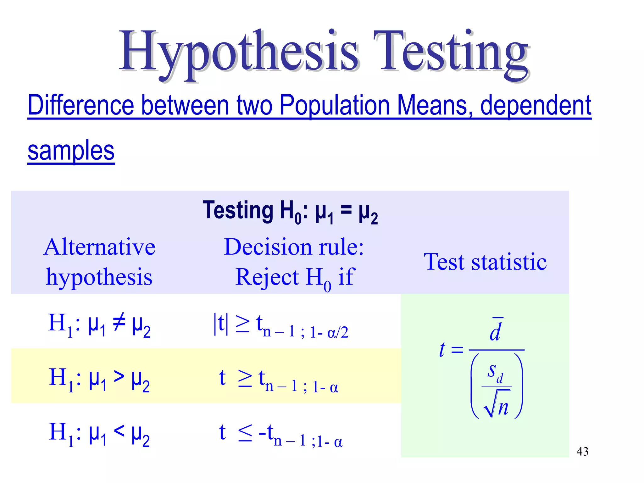
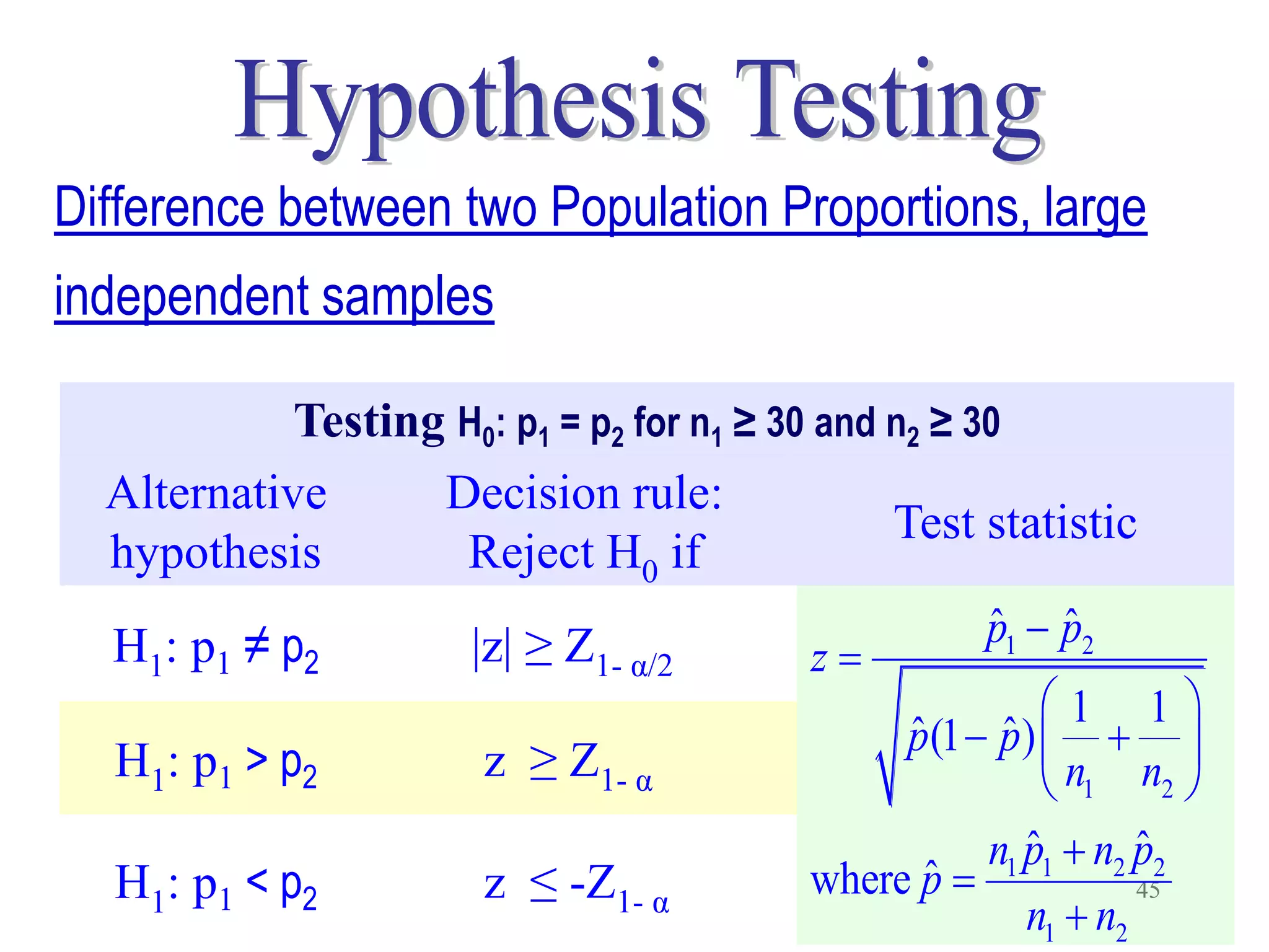
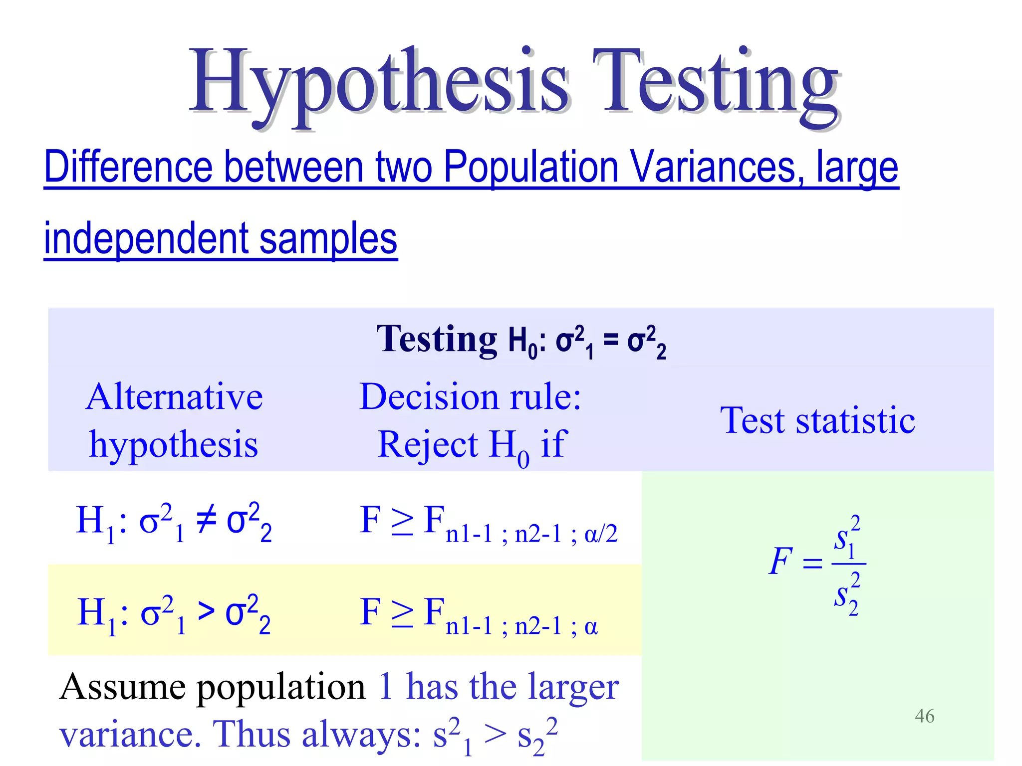
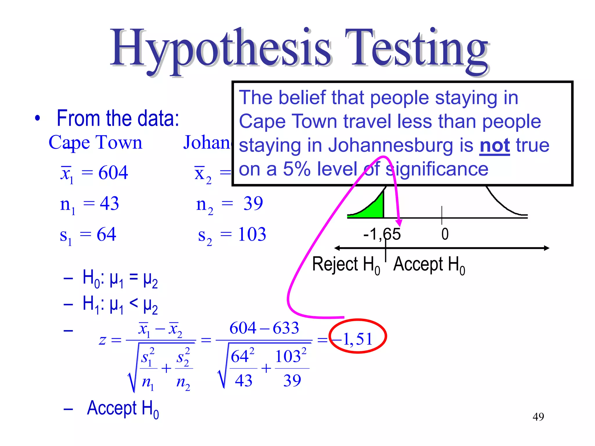
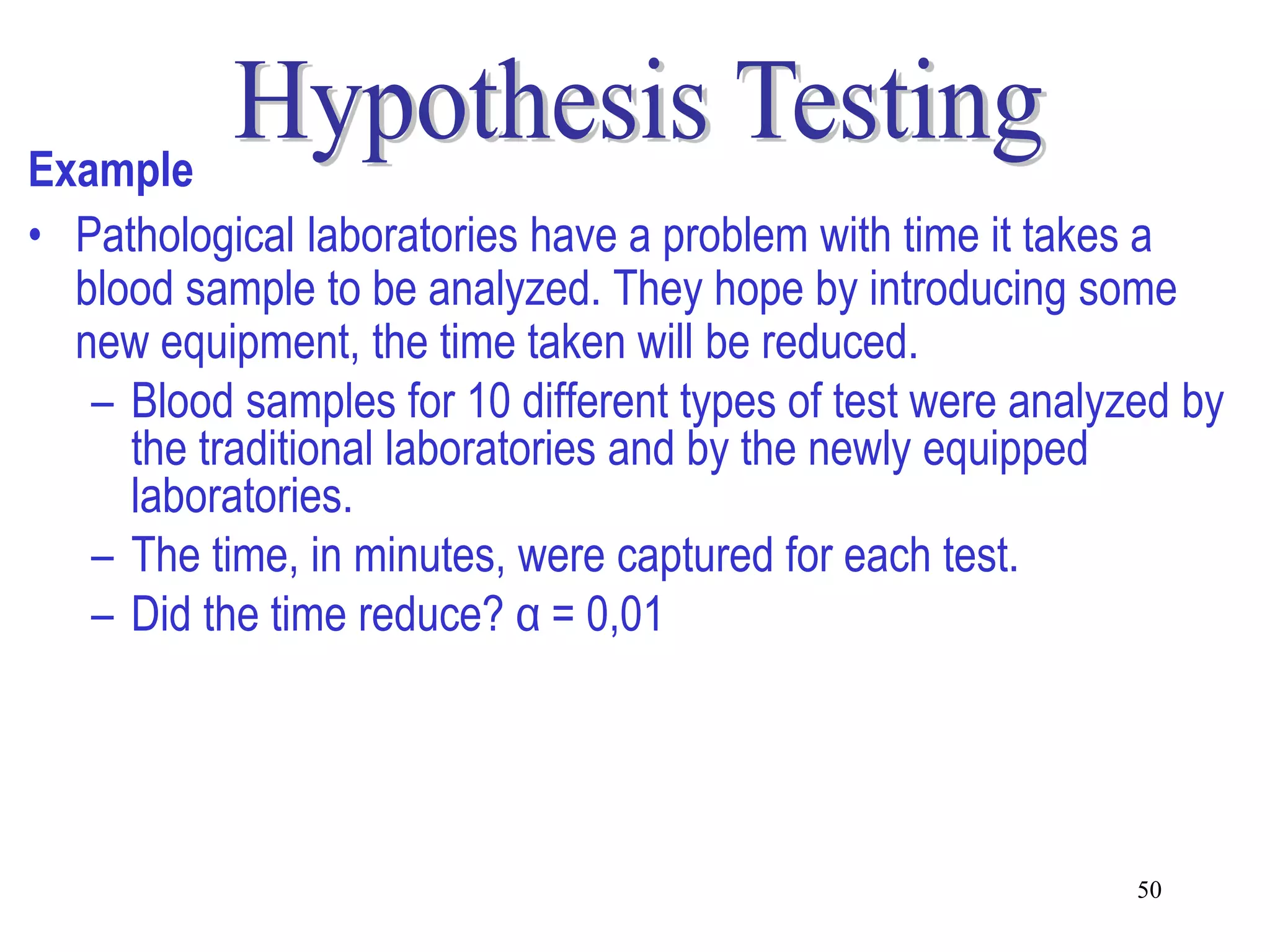
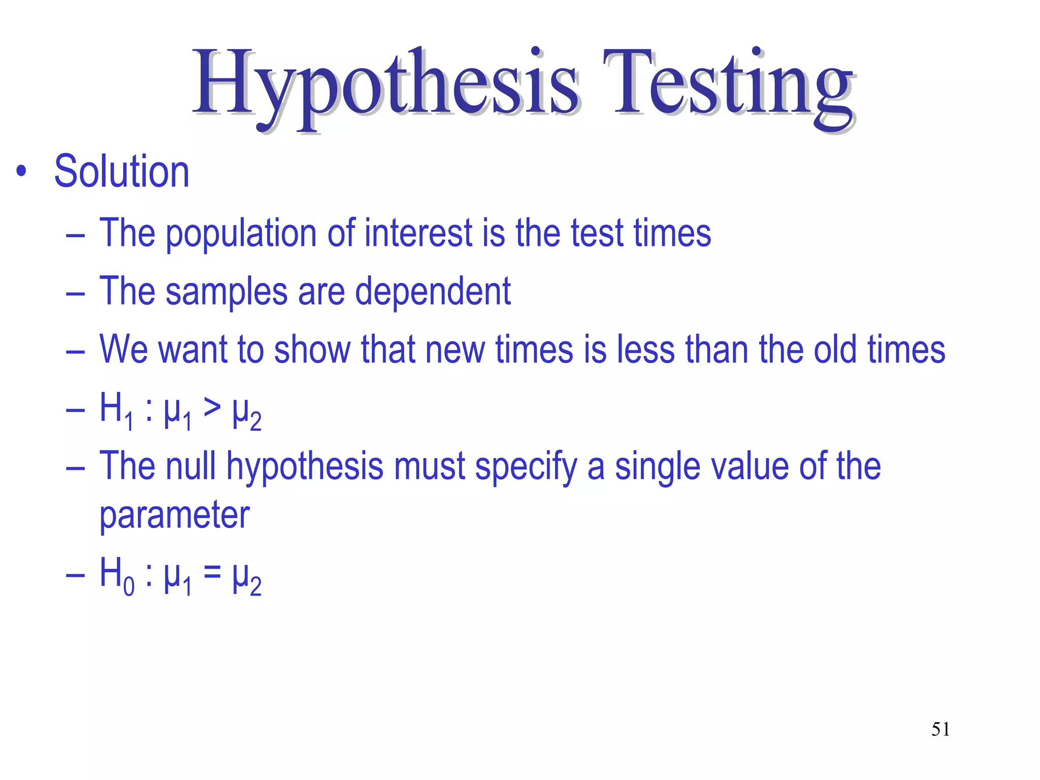
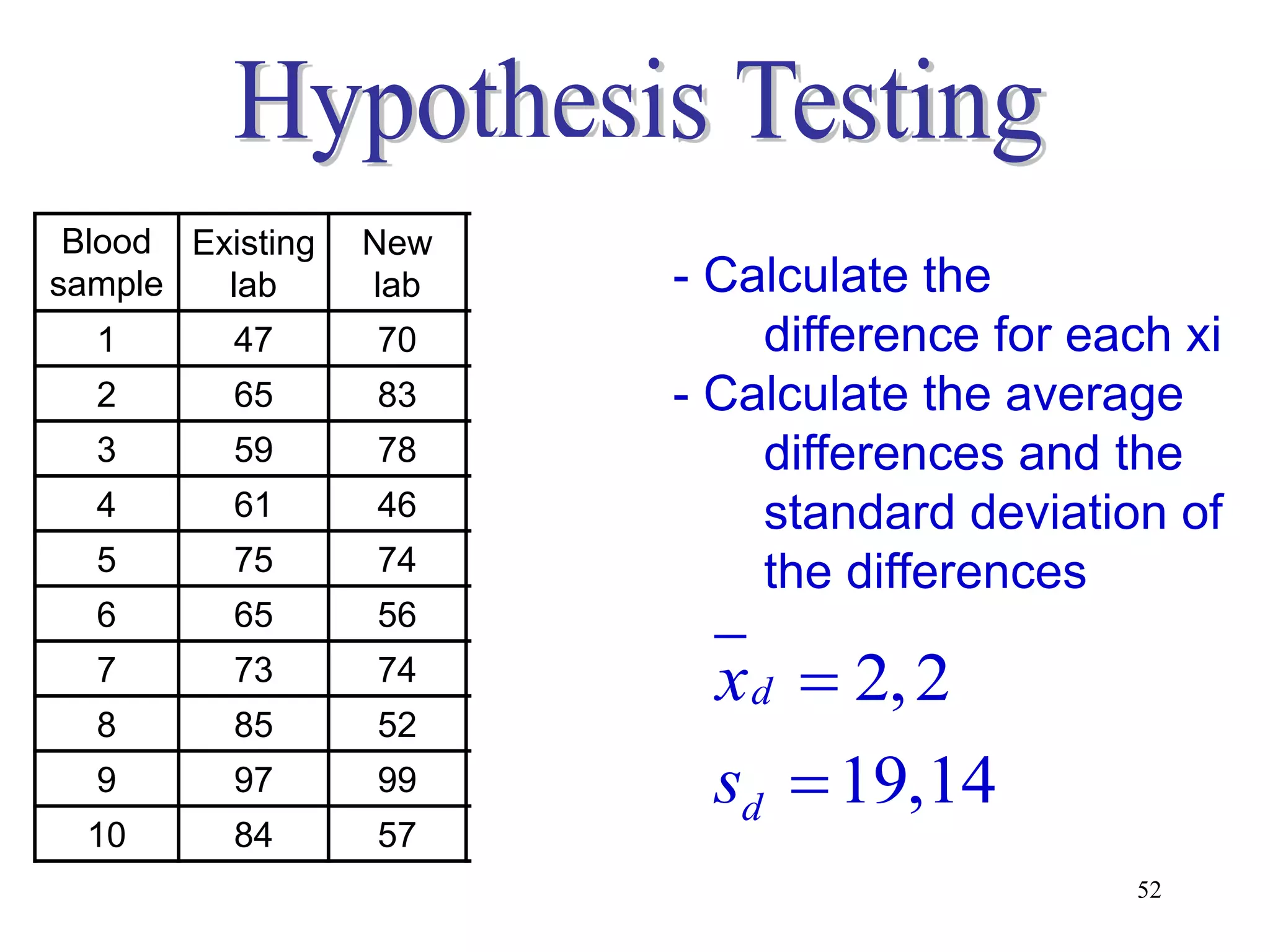
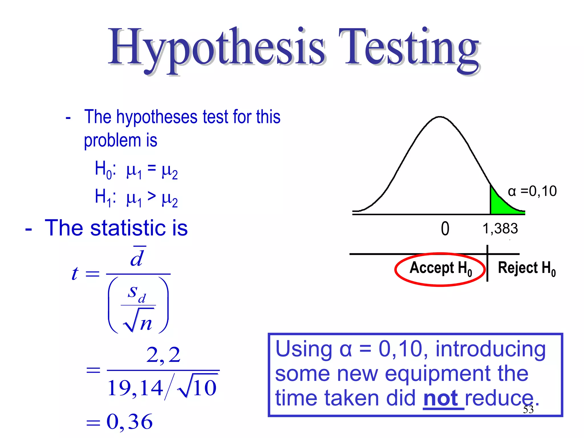
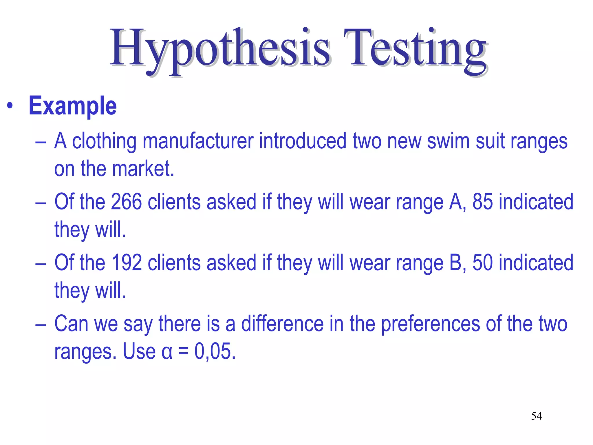
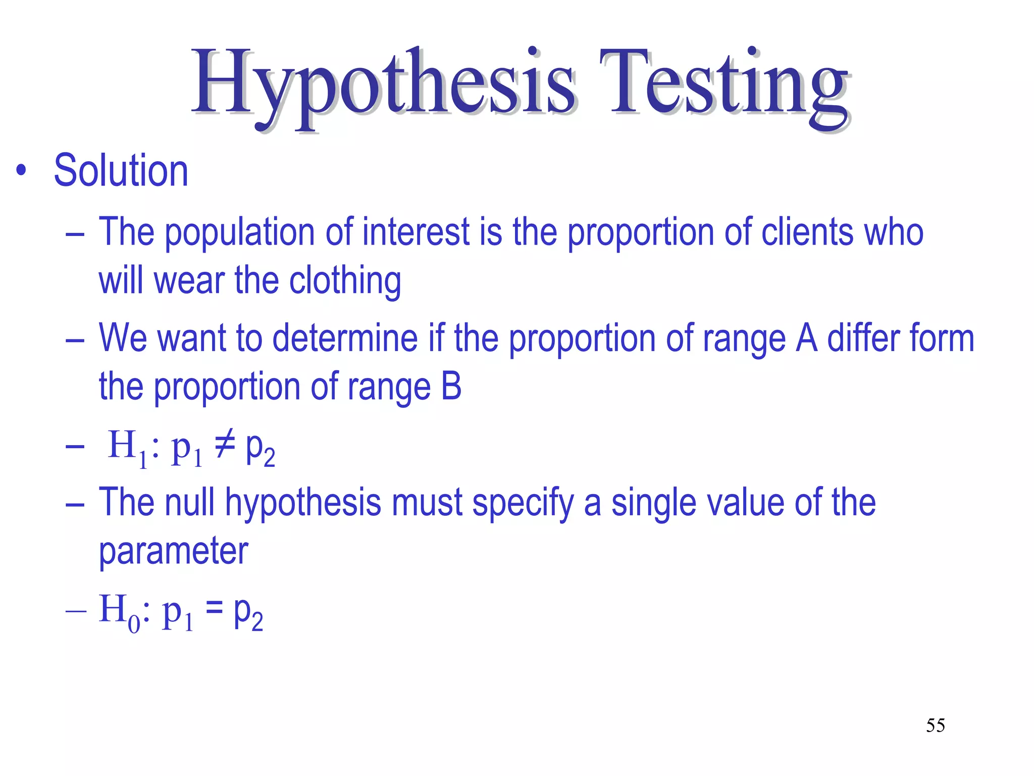
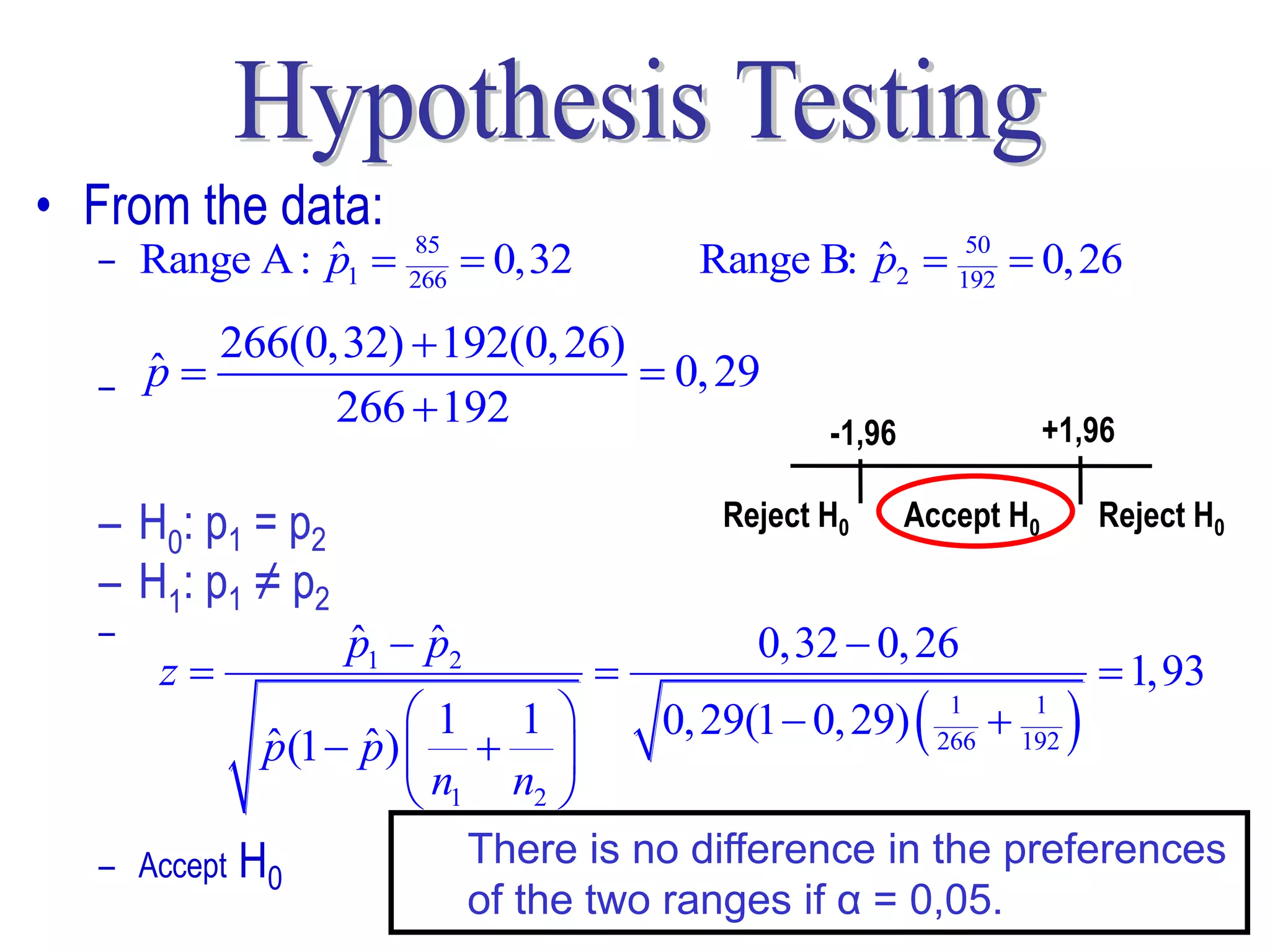
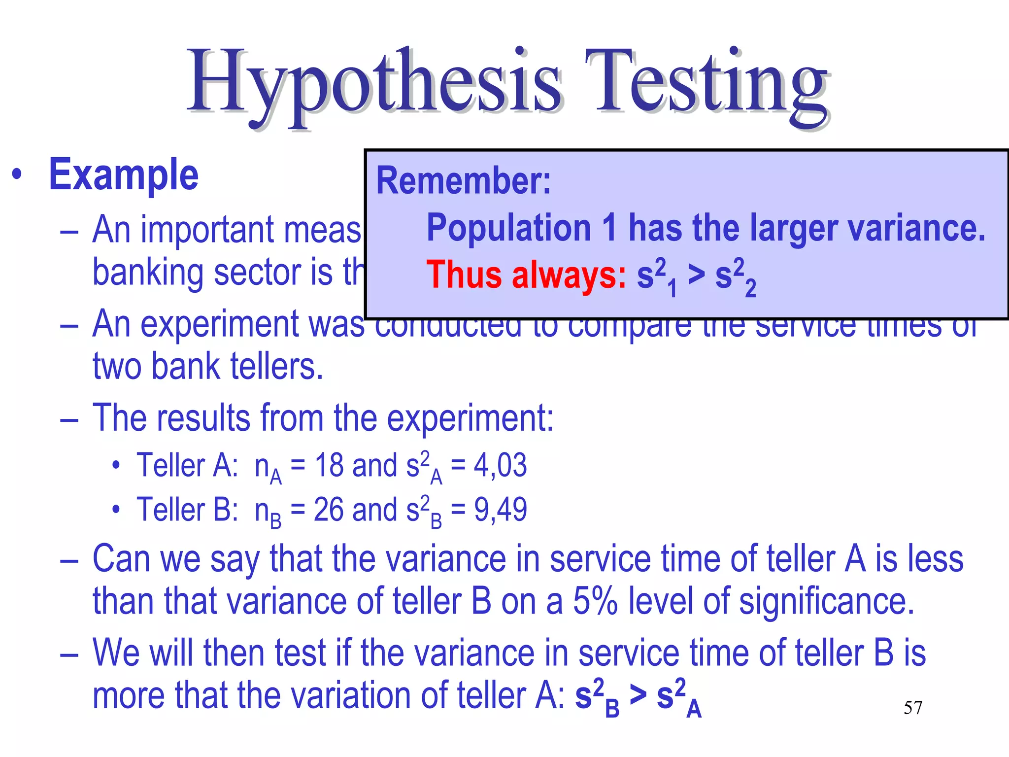
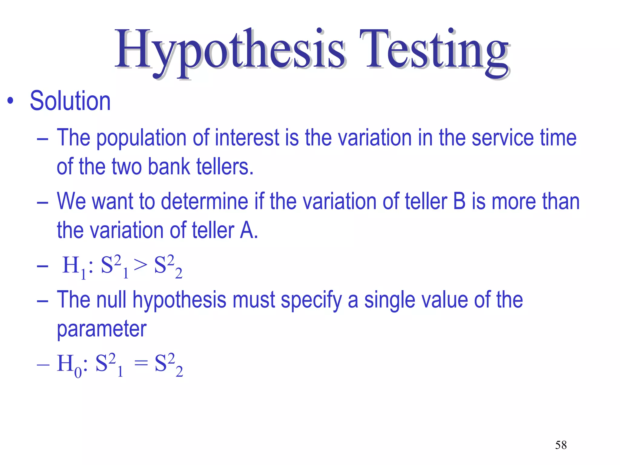
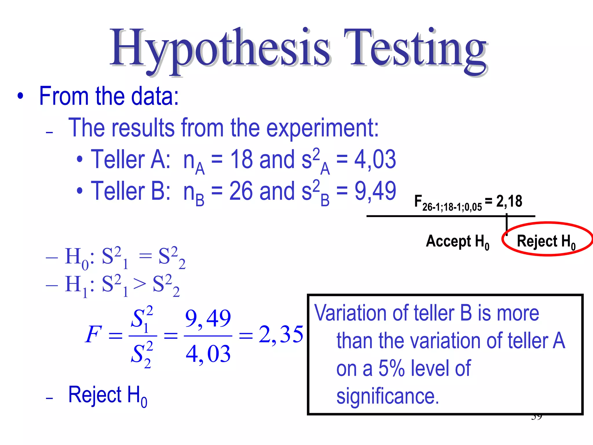
1
Data collection                 Raw data

                    Graphs                 Information
 Descriptive
  statistics      Measures
                  • location
                  • spread


                                    Estimation
                  Statistical                        Decision
                  inference                          making
                                    Hypothesis
                                      testing            2
• Hypothesis testing is a procedure for
  making inferences about a population
• A hypothesis test gives the opportunity
 to test whether a change has occurred
 or a real difference exists
• A hypothesis is a statement or claim that
  something is true
                                      H0 always contains = sign
  – Null hypothesis H0
     • No effect or no difference
     • Must be declared true/false
  – Alternative hypothesis H1
     • True if H0 found to be false
  – If H0 is false – reject H0 and accept H1
  – If H0 is true – accept H0 and reject H1
•   State the null and alternative hypotheses that would be used to test each
    of the following statements:-
•   A manufacturer claims that the average life of a transistor is at least 1000
    hours (h)
          H0: µ = 1000
          H1: µ > 1000
•   A pharmaceutical firm maintains that the average time for a certain drug
    to take effect is 15 mins
          H0: µ = 15
          H1: µ ≠ 15
•   The mean starting salary of graduates is higher than R50000 per annum
          H0: µ = 50000
          H1: µ > 50000
•    Hypothesis testing consists of 6 steps:

    1.   State the hypothesis
    2.   State the value of α
    3.   Calculate the test statistic
    4.   Determine the critical value
    5.   Make a decision
    6.   Draw conclusion


                                               6
Hypothesis Testing Step 1    One/Two populations
 State the hypothesis              Two tailed
                               H0: parameter = ?
                               H1: parameter ≠ ?
Ho – Null hypothesis
                                  Right tailed
H1 – Alternative Hypothesis    H0: parameter = ?
                               H1: parameter > ?
                                   Left tailed
                               H0: parameter = ?
                               H1: parameter < ?    7
Hypothesis Testing Step 2
State the value of α Decision          Actual situation
                                  H0 is true     H0 is false
                       Do not     Correct
                      reject H0   decision
                                                  Correct
                     Reject H0
                                                  decision


                                                         8
Hypothesis Testing Step 2
 State the value of α Decision               Actual situation
                                        H0 is true     H0 is false
    Two types of errors:
                            Do not      Correct       Type II error =
                           reject H0    decision            
                                       Type I error      Correct
                           Reject H0
                                          =             decision

α - Probability of Type I error
    Level of significance
    1%, 5%, 10%
    Determine critical value/s                                  9
LEVEL OF SIGNIFICANCE
 •   Probability (α) of committing a type I
     error is called the LEVEL OF
     SIGNIFICANCE
 •   α is specified before the test is
     performed
 •   You can control the Type I error by
     deciding, before the test is performed,
     what risk level you are willing to take in
     rejecting H0 when it is in fact true
 •   Researchers usually select α levels of
     0.05 or smaller
                                                  10
Hypothesis Testing Step 3
Calculate value of test statistic

There are different test statistics for testing:
•   Single population
    – Mean, proportion, variance
•   Difference between two population
    – Means, proportions, variances

                                                   11
REJECTION AND NON-REJECTION REGIONS

• To decide whether H0 will be rejected or not , a
  value, called the TEST STATISTIC has to be
  calculated by using certain sample results
• Distribution of test statistic often follows a normal
  or t distribution.
• Distribution can be divided into 2 regions:-
   – A region of rejection
   – A region of non- rejection
                                                     12
Hypothesis Testing Step 4
Determine the critical value/values
   Right tailed             Two tailed                 Left tailed
 H1: parameter > ?      H1: parameter ≠ ?            H1: parameter < ?


       H0                       H0                        H0
                  α   α/2                α/2     α


                               - Critical value – from tables 13
Hypothesis Testing Step 5
Make decision
   Right tailed             Two tailed                   Left tailed
 H1: parameter > ?      H1: parameter ≠ ?              H1: parameter < ?

                                 H0
       H0                                                   H0
                  α   α/2                    α/2   α

     Accept Rej             Rej Accept Rej              Rej Accept
      H0 H0                 H0 H0 H0                    H0 H0
                                                                     14
Hypothesis Testing Step 6
Draw conclusion
                                     Accept H0
                                        ?
                            H0
                                     Reject H0

                        ?? ?


                    Test statistic               15
STEPS OF A HYPOTHESIS TEST
Step 1   • State the null and alternative hypotheses
Step 2   • State the values of α
Step 3   • Calculate the value of the test statistic
Step 4   • Determine the critical value
Step 5   • Make a decision using decision rule or graph
Step 6   • Draw a conclusion
                                                          16
Concept Questions
• 1 – 12 page 261 textbook


                              17
Hypothesis test for Population Mean, n ≥ 30
- population need not be normally distributed
- sample will be approximately normal
                  Testing H0: μ = μ0 for n ≥ 30
    Alternative       Decision rule:
                                             Test statistic
    hypothesis         Reject H0 if
    H1: μ ≠ μ0           |z| ≥ Z1- α/2           x  0
                                              z
    H1: μ > μ0           z ≥ Z1- α                s 
                                                     
    H1: μ < μ0           z ≤ -Z1- α                n         18
                                                      Use σ if known
• Example
  – It will be cost effective to employee an additional staff
    member at a well known take away restaurant if the
    average sales for a day is more than R11 000 per day.
  – A sample of 60 days were selected and the average sales
    for the 60 days were R11 841 with a standard deviation of
    R1 630.
  – Test if it will be cost effective to employ an additional staff
    member.
  – Assume a normal distributed population. Use α = 0,05.
• Solution
  – The population of interest is the daily sales
  – We want to show that the average sales is more than
    R11 000 per day.
  – H1 : μ > 11 000
  – The null hypothesis must specify a single value of the
    parameter 
  – H0 : μ = 11 000
  – Need to test if R11 841( x ) is significant more than
    R11 000(μ)
• Solution             At α = 0,05 if it will be cost effective to
  – H0 : μ = 11 000    employ an additional staff member –
                       the average monthly income is more
  – H1 : μ > 11 000
                                    than R11 000
  – α = 0,05
   x  0 11841  11000                                        α = 0,05
z                        3,99
  – s         1630
                                                 0        z1-α
                                                            1,65
      n         60
                                                Accept H0      Reject H0
  – Reject H0

                           Critical value Z 1-α = Z 0.95 = 1.65
• Hypothesis test for Population Mean, n < 30
   – If σ is unknown we use s to estimate σ
   – We need to replace the normal distribution with the
     t-distribution with (n - 1) degrees of freedom

             Testing H0: μ = μ0 for n < 30
 Alternative      Decision rule:
                                         Test statistic
 hypothesis        Reject H0 if
 H1: μ ≠ μ0        |t| ≥ tn - 1;1- α/2       x  0
                                          t
  H1: μ > μ0        t ≥ tn-1;1- α             s 
                                                 
                                              n
  H1: μ < μ0        t ≤ -tn-1;1- α                         22
Concept Questions

Questions 13 – 19, page 267, textbook


                                        23
• Example
  – Health care is a major issue world wide. One of the
    concerns is the waiting time for patients at clinics.
  – Government claims that patients will wait less than 30
    minutes on average to see a doctor.
  – A random sample of 25 patients revealed that their average
    waiting time was 28 minutes with a standard deviation of 8
    minutes.
  – On a 1% level of significance can we say that the claim
    from government is correct?
                                                          24
• Solution
  – The population of interest is the waiting time at clinics
  – Want to test the claim that the waiting time is less than 30
    minutes
  – H1 : μ < 30
  – The null hypothesis must specify a single value of the
    parameter 
  – H0 : μ = 30
  – Need to test if 28( x ) is significant less than 30(μ)

                                                               25
• Solution                 At α = 0,01 we can not say that
  – H0 : μ = 30              the average waiting time at
  – H1 : μ < 30            clinics is less than 30 minutes
  – α = 0,01                        α = 0,01
     x  0 28  30
  t                    1, 25
  –     s        8
                                             -t1-α
                                               -2,492    0
        n        25
                                     Reject H0     Accept H0
  – Accept H0
                           tn-1;1-α = t24;0.99= -2.492

                                                               26
• Hypothesis testing for Population proportion
                          number of successes   x
  – Sample proportion p =
                      ˆ                       =
                             sample size        n

  – Proportion always between 0 and 1
                Testing H0: p = p0 for n ≥ 30
  Alternative        Decision rule:
                                          Test statistic
  hypothesis          Reject H0 if
   H1: p ≠ p0          |z| ≥ Z1- α/2             p  p0
                                                 ˆ
                                         z
   H1: p > p0           z ≥ Z1- α               p0 (1  p0 )
   H1: p < p0           z ≤ -Z1- α                   n         27
• Example
  – A market research company investigates the claim of a
    supplier that 35% of potential buyers are preferring their
    brand of milk
  – A survey was done in several supermarkets and it was
    found that 61 of the 145 shoppers indicated that they will
    buy the specific brand of milk
  – Assist the research company with the claim of the supplier
    on a 10% level of significance.

                                                           28
• Solution
  – The population of interest is the proportion of buyers
  – Want to test the claim that the proportion is 35% = 0,35
  –  H0 : p = 0,35
  – The alternative hypothesis must specify that the proportion
    is not 35%
  – H1 : p ≠ 0,35
  – Sample proportion p = number of successes = x  61  0, 42
                      ˆ
                                sample size        n   145

  – Need to test if 0,42 p  is significant different from 0,35(p)
                          ˆ
                                                               29
• Solution
                                     /2  0,05
At – = 0 : p = 0,35 not say
   α H 0,10 we can
that 35%p ≠the clients will
   – H1 : of 0,35                            -z-1,65                z1-/2
                                                1-/2               +1,65
  prefer the brand of milk
   – α = 0,10
                                       Reject H0        Accept H0       Reject H0

              p  p0
              ˆ               0, 42  0,35
     z                                      1, 76
             p0 (1  p0 )     0,35(1  0,35)
                  n                145
                                        Z1-α/2 = Z0.95 = +/- 1.65
  – Reject H0
                                                                             30
• Hypothesis testing for Population Variance
  – Draw conclusions about variability in population
  – Χ2 –distribution with (n - 1) degrees of freedom

                  Testing H0: σ2 = σ20
  Alternative      Decision rule:
                                       Test statistic
  hypothesis        Reject H0 if
                 Χ2 ≤ Χ2n-1;α/2 or
  H1: σ2 ≠ σ20                                 (n  1) s 2
                 Χ2 ≥ Χ2n-1;1- α/2      2 
  H1: σ2 > σ20   Χ2 ≥ Χ2n-1;1- α                   02
  H1: σ2 < σ20   Χ2 ≤ Χ2n-1;α                                31
Concept Questions
• Questions 20 – 24 page 272


                               32
• Example
  – The variation in the content of a 340ml can of beer should
    not be more than 10ml2.
  – To test the validity of this, 25 cans of beers revealed a
    variance of 12ml2.
  – On a 5% level of significance can we say the variation in
    the content of the cans is too large?


                                                           33
• Solution
  –   The population of interest is the variation in content
  –   Want to test the claim that the variance is more than 10ml2
  –   H1 : σ2 > 10
  –   The null hypothesis must specify that the variance is 10ml2
  –   H0 : σ2 = 10
  –   Need to test if 12(s2) is significant more than 10(σ2)


                                                            34
• Solution
   – H0 : σ2 = 10                                                        0,05

   – H1 : σ2 > 10
   – α = 0,05                                                    Χ2n – 1; 1-α
                                                                  +36,42
             (n  1) s   2
                                (25  1)12
        
        2
                                            28,8        Accept H0    Reject H0
                     02           10
                                    At α = 0,05 we can not say
    – Accept H0                        that the variation in the
                                    content of the cans is more
Χ n-1; 1-α = Χ 24; 0.95 = 36.42
 2            2
                                              than 10ml2
                                                                           35
• Hypothesis tests for comparing two
  Populations             Drawn from different
  – Difference between two means
                             samples, samples
                               have no relation
     • Independent samples
        – Large samples
        – Small samples         Samples are
     • Dependent samples          related

  – Difference between two proportions
  – Difference between two variances              36
• Hypothesis tests for comparing two Populations
  –   H0: Population 1 parameter = Population 2 parameter
  –   H1: Population 1 parameter ≠ Population 2 parameter
  –   H1: Population 1 parameter > Population 2 parameter
  –   H1: Population 1 parameter < Population 2 parameter


                     μ1 / σ21 / p1           μ2 / σ22 / p2
Difference between two Population Means,
independent samples, n1 ≥ 30 and n2 ≥ 30

         Testing H0: μ1 = μ2 for n1 ≥ 30 and n2 ≥ 30
   Alternative      Decision rule:
                                           Test statistic
   hypothesis        Reject H0 if
   H1: μ1 ≠ μ2        |z| ≥ Z1- α/2              x1  x2
                                          z
   H1: μ1 > μ2         z ≥ Z1- α                  s12 s2
                                                       2
                                                     
   H1: μ1 < μ2         z ≤ -Z1- α                 n1 n2
                                                              38
                                           Use σ12 and σ22 if known
Example
 A leading television manufacturer purchases
cathode ray tubes from 2 businesses (A and B). A
random sample of 36 cathode ray tubes from
business A showed a mean lifetime of 7.2 years
and a std dev of 0.8 years, while a random sample
of 40 cathode ray tubes from business B showed a
mean lifetime of 6.7 years and a std dev of 0.7 yrs.
Test at a 1% significance level whether the mean
lifetime of the cathode ray tubes from business A is
longer than the mean lifetime of business B
                                                  39
Answer
    Company A: n1 = 36, x1 = 7,2 and s1 = 0,8.
    Company B: n2 = 40, x 2 = 6,7 and s2 = 0,7.
    H0: 1 = 2
                
    H1: 1 > 2
                
     = 0,01
         x1  x 2
    z=
         s12 s2
              2
            
         n1 n 2
            7,2  6,7
     =
         0,8        0,7
                2           2

                   
           36          40
         0,5
     =
       0,1733
      = 2,8852
     Z1 = Z0,99 = 2,33

    Therefore, reject H0.
    There is enough evidence to say that the mean lifetime of the tubes from Company A is longer
    than that of Company B.


                                                                                       40
Difference between two Population Means, independent
samples, n1 < 30 and n2 < 30

         Testing H0: μ1 = μ2 for n1 < 30 and n2 < 30
 Alternative       Decision rule:
                                             Test statistic
 hypothesis          Reject H0 if
                                                       x1  x2
 H1: μ1 ≠ μ2       |t| ≥ tn1 + n2 – 2 ; 1- α/2   t                    with
                                                          1 2
                                                    sp      
                                                         n1 n2
 H1: μ1 > μ2        t ≥ tn1 + n2 – 2 ; 1- α
                                                 sp 
                                                         n1  1 s12   n2  1 s22
 H1: μ1 < μ2        t ≤ -tn1 + n2 – 2 ;1- α                    n1  n2  2
                                                                              41
Difference between two Population Means, dependent
samples – pairs of observations
                                      Observation
                   1           2         3      ----------              n
   Sample 1       X11         X12        X13       - - - - - - - - - - X1n
   Sample 2       X21         X22        X23       - - - - - - - - - - X2n
                   d1          d2         d3                          dn
 Difference (d)
                  (X11 - X21) (X12 - X22) (X13 – X23)          (X1n - X2n)


                                         d                 d 
                                                                    2
         1
                                               2
                                                      1

      d   d and sd                                  n

         n                                         n 1                 42
Difference between two Population Means, dependent
samples

               Testing H0: μ1 = μ2
 Alternative     Decision rule:
                                        Test statistic
 hypothesis       Reject H0 if
 H1: μ1 ≠ μ2    |t| ≥ tn – 1 ; 1- α/2             d
                                         t
 H1: μ1 > μ2    t ≥ tn – 1 ; 1- α                sd 
                                                    
                                                  n
 H1: μ1 < μ2    t ≤ -tn – 1 ;1- α
                                                         43
Concept Questions
  Questions 25 – 29 p 283, textbook


                                      44
Difference between two Population Proportions, large
independent samples

            Testing H0: p1 = p2 for n1 ≥ 30 and n2 ≥ 30
  Alternative      Decision rule:
                                                Test statistic
  hypothesis        Reject H0 if
  H1: p1 ≠ p2          |z| ≥ Z1- α/2                 p1  p2
                                                     ˆ ˆ
                                           z
                                                        1 1
                                               p(1  p)   
                                               ˆ     ˆ
  H1: p1 > p2          z ≥ Z1- α                         n1 n2 
                                                    n1 p1  n2 p2
                                                       ˆ       ˆ
  H1: p1 < p2          z ≤ -Z1- α         where p 
                                                ˆ              45
                                                       n1  n2
Difference between two Population Variances, large
independent samples

                   Testing H0: σ21 = σ22
  Alternative     Decision rule:
                                           Test statistic
  hypothesis       Reject H0 if
 H1: σ21 ≠ σ22    F ≥ Fn1-1 ; n2-1 ; α/2        s12
                                              F 2
 H1: σ21 > σ22    F ≥ Fn1-1 ; n2-1 ; α          s2

Assume population 1 has the larger
                                                        46
variance. Thus always: s21 > s22
• Example
• There is a belief that people staying in Cape Town
  travel less than people staying in Johannesburg.
   – Random samples of 43 people in Cape Town and 39
     in Johannesburg were drawn.
   – For each person the distance travelled during
     October were recorded.
   – Test the belief on a 5% level of significance


                                                   47
• Solution
  – The population of interest is the km travelled
  – Samples are large and independent
  – We want to show that Cape Town travel less than
    Johannesburg
  – H1 : μ1 < μ2
  – The null hypothesis must specify a single value of the
    parameter 
  – H0 : μ1 = μ2

                                                             48
The belief that people staying in
• From the data:        Cape Town travel less than people
   –
 Cape Town       Johanesburg in Johannesburg is not true
                        staying
  x1 = 604        x 2 = 633a 5% level of significance
                        on
  n1 = 43           n 2 = 39
  s1 = 64           s 2 = 103           -1,65     0
                                  Reject H0 Accept H0
   – H0: μ1 = μ2
   – H1: μ1 < μ2
   – z  x1  x2  604  633  1,51
               2 2   2      2
            s1 s2       64 103
                          
            n1 n2       43   39
   – Accept H0                                          49
Example
• Pathological laboratories have a problem with time it takes a
  blood sample to be analyzed. They hope by introducing some
  new equipment, the time taken will be reduced.
   – Blood samples for 10 different types of test were analyzed by
     the traditional laboratories and by the newly equipped
     laboratories.
   – The time, in minutes, were captured for each test.
   – Did the time reduce? α = 0,01


                                                             50
• Solution
  – The population of interest is the test times
  – The samples are dependent
  – We want to show that new times is less than the old times
  – H1 : μ1 > μ2
  – The null hypothesis must specify a single value of the
    parameter
  – H0 : μ1 = μ2


                                                           51
Blood Existing   New
                        Difference   - Calculate the
sample   lab      lab
  1       47      70       -23           difference for each xi
  2       65      83       -18       - Calculate the average
  3       59      78       -19           differences and the
  4       61      46       15            standard deviation of
  5       75      74        1            the differences
  6       65      56        9
  7       73      74        -1
                                      x d  2, 2
  8       85      52       33
  9       97      99        -2        sd  19,14
  10      84      57       27
                                                          52
- The hypotheses test for this
     problem is
      H0: 1 = 2
      H1: 1 > 2                                            α =0,10

- The statistic is                               0       1,383
                                                         t0.90,9

           d
    t                                       Accept H0      Reject H0
         sd 
             
         n
             2, 2               Using α = 0,10, introducing
                               some new equipment the
        19,14 10                time taken did not reduce.
                                                         53
      0, 36
• Example
  – A clothing manufacturer introduced two new swim suit ranges
    on the market.
  – Of the 266 clients asked if they will wear range A, 85 indicated
    they will.
  – Of the 192 clients asked if they will wear range B, 50 indicated
    they will.
  – Can we say there is a difference in the preferences of the two
    ranges. Use α = 0,05.

                                                              54
• Solution
  – The population of interest is the proportion of clients who
    will wear the clothing
  – We want to determine if the proportion of range A differ form
    the proportion of range B
  – H1: p1 ≠ p2
  – The null hypothesis must specify a single value of the
    parameter
  – H0: p1 = p2

                                                             55
• From the data:
  –   Range A : p1  266  0,32
                ˆ    85
                                      Range B: p2  192  0, 26
                                               ˆ     50


         266(0,32)  192(0, 26)
  –   p
      ˆ                          0, 29
               266  192                                          +1,96
                                              -1,96

  – H0: p1 = p2                        Reject H0      Accept H0        Reject H0

  – H1: p1 ≠ p2
  –               p1  p2
                  ˆ ˆ                    0,32  0, 26
       z                                                              1,93
                       1 1
              p(1  p)   
              ˆ     ˆ                                 
                                      0, 29(1  0, 29) 266  192
                                                        1     1
                                                                   
                        n1 n2 
  –   Accept H0            There is no difference in the preferences
                           of the two ranges if α = 0,05.        56
• Example               Remember:
  – An important measure to determine 1 has the largerin the
                            Population service delivery variance.
    banking sector is the variability in the service 2times.
                            Thus always: s21 > s 2
  – An experiment was conducted to compare the service times of
    two bank tellers.
  – The results from the experiment:
     • Teller A: nA = 18 and s2A = 4,03
     • Teller B: nB = 26 and s2B = 9,49
  – Can we say that the variance in service time of teller A is less
    than that variance of teller B on a 5% level of significance.
  – We will then test if the variance in service time of teller B is
    more that the variation of teller A: s2B > s2A                57
• Solution
  – The population of interest is the variation in the service time
    of the two bank tellers.
  – We want to determine if the variation of teller B is more than
    the variation of teller A.
  – H1: S21 > S22
  – The null hypothesis must specify a single value of the
    parameter
  – H0: S21 = S22


                                                               58
• From the data:
   – The results from the experiment:

      • Teller A: nA = 18 and s2A = 4,03
      • Teller B: nB = 26 and s2B = 9,49    F26-1;18-1;0,05 = 2,18

                                              Accept H0         Reject H0
   –   H0: 1 = S22
          S2
   –   H1: S21 > S22
            S   2
                9, 49       Variation of teller B is more
         F   1
                2
                       2,35 than the variation of teller A
            S   4, 03
               2
                                   on a 5% level of
   –   Reject H0                   significance.
                                                                     59
Concept Questions
• Questions 30 -31, p 289, textbook


                                      60
HOMEWORK
•   Self review test, p289
•   Izmivo
•   Revision test
•   Supplementary Questions p292 – 298


                                         61

Statistics lecture 9 (chapter 8)

  • 1.
  • 2.
    Data collection Raw data Graphs Information Descriptive statistics Measures • location • spread Estimation Statistical Decision inference making Hypothesis testing 2
  • 3.
    • Hypothesis testingis a procedure for making inferences about a population • A hypothesis test gives the opportunity to test whether a change has occurred or a real difference exists
  • 4.
    • A hypothesisis a statement or claim that something is true H0 always contains = sign – Null hypothesis H0 • No effect or no difference • Must be declared true/false – Alternative hypothesis H1 • True if H0 found to be false – If H0 is false – reject H0 and accept H1 – If H0 is true – accept H0 and reject H1
  • 5.
    State the null and alternative hypotheses that would be used to test each of the following statements:- • A manufacturer claims that the average life of a transistor is at least 1000 hours (h) H0: µ = 1000 H1: µ > 1000 • A pharmaceutical firm maintains that the average time for a certain drug to take effect is 15 mins H0: µ = 15 H1: µ ≠ 15 • The mean starting salary of graduates is higher than R50000 per annum H0: µ = 50000 H1: µ > 50000
  • 6.
    Hypothesis testing consists of 6 steps: 1. State the hypothesis 2. State the value of α 3. Calculate the test statistic 4. Determine the critical value 5. Make a decision 6. Draw conclusion 6
  • 7.
    Hypothesis Testing Step1 One/Two populations State the hypothesis Two tailed H0: parameter = ? H1: parameter ≠ ? Ho – Null hypothesis Right tailed H1 – Alternative Hypothesis H0: parameter = ? H1: parameter > ? Left tailed H0: parameter = ? H1: parameter < ? 7
  • 8.
    Hypothesis Testing Step2 State the value of α Decision Actual situation H0 is true H0 is false Do not Correct reject H0 decision Correct Reject H0 decision 8
  • 9.
    Hypothesis Testing Step2 State the value of α Decision Actual situation H0 is true H0 is false Two types of errors: Do not Correct Type II error = reject H0 decision  Type I error Correct Reject H0 = decision α - Probability of Type I error Level of significance 1%, 5%, 10% Determine critical value/s 9
  • 10.
    LEVEL OF SIGNIFICANCE • Probability (α) of committing a type I error is called the LEVEL OF SIGNIFICANCE • α is specified before the test is performed • You can control the Type I error by deciding, before the test is performed, what risk level you are willing to take in rejecting H0 when it is in fact true • Researchers usually select α levels of 0.05 or smaller 10
  • 11.
    Hypothesis Testing Step3 Calculate value of test statistic There are different test statistics for testing: • Single population – Mean, proportion, variance • Difference between two population – Means, proportions, variances 11
  • 12.
    REJECTION AND NON-REJECTIONREGIONS • To decide whether H0 will be rejected or not , a value, called the TEST STATISTIC has to be calculated by using certain sample results • Distribution of test statistic often follows a normal or t distribution. • Distribution can be divided into 2 regions:- – A region of rejection – A region of non- rejection 12
  • 13.
    Hypothesis Testing Step4 Determine the critical value/values Right tailed Two tailed Left tailed H1: parameter > ? H1: parameter ≠ ? H1: parameter < ? H0 H0 H0 α α/2 α/2 α - Critical value – from tables 13
  • 14.
    Hypothesis Testing Step5 Make decision Right tailed Two tailed Left tailed H1: parameter > ? H1: parameter ≠ ? H1: parameter < ? H0 H0 H0 α α/2 α/2 α Accept Rej Rej Accept Rej Rej Accept H0 H0 H0 H0 H0 H0 H0 14
  • 15.
    Hypothesis Testing Step6 Draw conclusion Accept H0 ? H0 Reject H0 ?? ? Test statistic 15
  • 16.
    STEPS OF AHYPOTHESIS TEST Step 1 • State the null and alternative hypotheses Step 2 • State the values of α Step 3 • Calculate the value of the test statistic Step 4 • Determine the critical value Step 5 • Make a decision using decision rule or graph Step 6 • Draw a conclusion 16
  • 17.
    Concept Questions • 1– 12 page 261 textbook 17
  • 18.
    Hypothesis test forPopulation Mean, n ≥ 30 - population need not be normally distributed - sample will be approximately normal Testing H0: μ = μ0 for n ≥ 30 Alternative Decision rule: Test statistic hypothesis Reject H0 if H1: μ ≠ μ0 |z| ≥ Z1- α/2 x  0 z H1: μ > μ0 z ≥ Z1- α  s    H1: μ < μ0 z ≤ -Z1- α  n 18 Use σ if known
  • 19.
    • Example – It will be cost effective to employee an additional staff member at a well known take away restaurant if the average sales for a day is more than R11 000 per day. – A sample of 60 days were selected and the average sales for the 60 days were R11 841 with a standard deviation of R1 630. – Test if it will be cost effective to employ an additional staff member. – Assume a normal distributed population. Use α = 0,05.
  • 20.
    • Solution – The population of interest is the daily sales – We want to show that the average sales is more than R11 000 per day. – H1 : μ > 11 000 – The null hypothesis must specify a single value of the parameter  – H0 : μ = 11 000 – Need to test if R11 841( x ) is significant more than R11 000(μ)
  • 21.
    • Solution At α = 0,05 if it will be cost effective to – H0 : μ = 11 000 employ an additional staff member – the average monthly income is more – H1 : μ > 11 000 than R11 000 – α = 0,05 x  0 11841  11000 α = 0,05 z   3,99 – s  1630   0 z1-α 1,65  n 60 Accept H0 Reject H0 – Reject H0 Critical value Z 1-α = Z 0.95 = 1.65
  • 22.
    • Hypothesis testfor Population Mean, n < 30 – If σ is unknown we use s to estimate σ – We need to replace the normal distribution with the t-distribution with (n - 1) degrees of freedom Testing H0: μ = μ0 for n < 30 Alternative Decision rule: Test statistic hypothesis Reject H0 if H1: μ ≠ μ0 |t| ≥ tn - 1;1- α/2 x  0 t H1: μ > μ0 t ≥ tn-1;1- α  s     n H1: μ < μ0 t ≤ -tn-1;1- α 22
  • 23.
    Concept Questions Questions 13– 19, page 267, textbook 23
  • 24.
    • Example – Health care is a major issue world wide. One of the concerns is the waiting time for patients at clinics. – Government claims that patients will wait less than 30 minutes on average to see a doctor. – A random sample of 25 patients revealed that their average waiting time was 28 minutes with a standard deviation of 8 minutes. – On a 1% level of significance can we say that the claim from government is correct? 24
  • 25.
    • Solution – The population of interest is the waiting time at clinics – Want to test the claim that the waiting time is less than 30 minutes – H1 : μ < 30 – The null hypothesis must specify a single value of the parameter  – H0 : μ = 30 – Need to test if 28( x ) is significant less than 30(μ) 25
  • 26.
    • Solution At α = 0,01 we can not say that – H0 : μ = 30 the average waiting time at – H1 : μ < 30 clinics is less than 30 minutes – α = 0,01 α = 0,01 x  0 28  30 t   1, 25 –  s  8   -t1-α -2,492 0  n 25 Reject H0 Accept H0 – Accept H0 tn-1;1-α = t24;0.99= -2.492 26
  • 27.
    • Hypothesis testingfor Population proportion number of successes x – Sample proportion p = ˆ = sample size n – Proportion always between 0 and 1 Testing H0: p = p0 for n ≥ 30 Alternative Decision rule: Test statistic hypothesis Reject H0 if H1: p ≠ p0 |z| ≥ Z1- α/2 p  p0 ˆ z H1: p > p0 z ≥ Z1- α p0 (1  p0 ) H1: p < p0 z ≤ -Z1- α n 27
  • 28.
    • Example – A market research company investigates the claim of a supplier that 35% of potential buyers are preferring their brand of milk – A survey was done in several supermarkets and it was found that 61 of the 145 shoppers indicated that they will buy the specific brand of milk – Assist the research company with the claim of the supplier on a 10% level of significance. 28
  • 29.
    • Solution – The population of interest is the proportion of buyers – Want to test the claim that the proportion is 35% = 0,35 – H0 : p = 0,35 – The alternative hypothesis must specify that the proportion is not 35% – H1 : p ≠ 0,35 – Sample proportion p = number of successes = x  61  0, 42 ˆ sample size n 145 – Need to test if 0,42 p  is significant different from 0,35(p) ˆ 29
  • 30.
    • Solution /2  0,05 At – = 0 : p = 0,35 not say α H 0,10 we can that 35%p ≠the clients will – H1 : of 0,35 -z-1,65 z1-/2 1-/2 +1,65 prefer the brand of milk – α = 0,10 Reject H0 Accept H0 Reject H0 p  p0 ˆ 0, 42  0,35 z   1, 76 p0 (1  p0 ) 0,35(1  0,35) n 145 Z1-α/2 = Z0.95 = +/- 1.65 – Reject H0 30
  • 31.
    • Hypothesis testingfor Population Variance – Draw conclusions about variability in population – Χ2 –distribution with (n - 1) degrees of freedom Testing H0: σ2 = σ20 Alternative Decision rule: Test statistic hypothesis Reject H0 if Χ2 ≤ Χ2n-1;α/2 or H1: σ2 ≠ σ20 (n  1) s 2 Χ2 ≥ Χ2n-1;1- α/2 2  H1: σ2 > σ20 Χ2 ≥ Χ2n-1;1- α  02 H1: σ2 < σ20 Χ2 ≤ Χ2n-1;α 31
  • 32.
    Concept Questions • Questions20 – 24 page 272 32
  • 33.
    • Example – The variation in the content of a 340ml can of beer should not be more than 10ml2. – To test the validity of this, 25 cans of beers revealed a variance of 12ml2. – On a 5% level of significance can we say the variation in the content of the cans is too large? 33
  • 34.
    • Solution – The population of interest is the variation in content – Want to test the claim that the variance is more than 10ml2 – H1 : σ2 > 10 – The null hypothesis must specify that the variance is 10ml2 – H0 : σ2 = 10 – Need to test if 12(s2) is significant more than 10(σ2) 34
  • 35.
    • Solution – H0 : σ2 = 10   0,05 – H1 : σ2 > 10 – α = 0,05 Χ2n – 1; 1-α +36,42 (n  1) s 2 (25  1)12   2   28,8 Accept H0 Reject H0  02 10 At α = 0,05 we can not say – Accept H0 that the variation in the content of the cans is more Χ n-1; 1-α = Χ 24; 0.95 = 36.42 2 2 than 10ml2 35
  • 36.
    • Hypothesis testsfor comparing two Populations Drawn from different – Difference between two means samples, samples have no relation • Independent samples – Large samples – Small samples Samples are • Dependent samples related – Difference between two proportions – Difference between two variances 36
  • 37.
    • Hypothesis testsfor comparing two Populations – H0: Population 1 parameter = Population 2 parameter – H1: Population 1 parameter ≠ Population 2 parameter – H1: Population 1 parameter > Population 2 parameter – H1: Population 1 parameter < Population 2 parameter μ1 / σ21 / p1 μ2 / σ22 / p2
  • 38.
    Difference between twoPopulation Means, independent samples, n1 ≥ 30 and n2 ≥ 30 Testing H0: μ1 = μ2 for n1 ≥ 30 and n2 ≥ 30 Alternative Decision rule: Test statistic hypothesis Reject H0 if H1: μ1 ≠ μ2 |z| ≥ Z1- α/2 x1  x2 z H1: μ1 > μ2 z ≥ Z1- α s12 s2 2  H1: μ1 < μ2 z ≤ -Z1- α n1 n2 38 Use σ12 and σ22 if known
  • 39.
    Example A leadingtelevision manufacturer purchases cathode ray tubes from 2 businesses (A and B). A random sample of 36 cathode ray tubes from business A showed a mean lifetime of 7.2 years and a std dev of 0.8 years, while a random sample of 40 cathode ray tubes from business B showed a mean lifetime of 6.7 years and a std dev of 0.7 yrs. Test at a 1% significance level whether the mean lifetime of the cathode ray tubes from business A is longer than the mean lifetime of business B 39
  • 40.
    Answer Company A: n1 = 36, x1 = 7,2 and s1 = 0,8. Company B: n2 = 40, x 2 = 6,7 and s2 = 0,7. H0: 1 = 2  H1: 1 > 2   = 0,01 x1  x 2 z= s12 s2 2  n1 n 2 7,2  6,7 = 0,8 0,7 2 2   36 40 0,5 = 0,1733  = 2,8852 Z1 = Z0,99 = 2,33  Therefore, reject H0. There is enough evidence to say that the mean lifetime of the tubes from Company A is longer than that of Company B. 40
  • 41.
    Difference between twoPopulation Means, independent samples, n1 < 30 and n2 < 30 Testing H0: μ1 = μ2 for n1 < 30 and n2 < 30 Alternative Decision rule: Test statistic hypothesis Reject H0 if x1  x2 H1: μ1 ≠ μ2 |t| ≥ tn1 + n2 – 2 ; 1- α/2 t with 1 2 sp  n1 n2 H1: μ1 > μ2 t ≥ tn1 + n2 – 2 ; 1- α sp   n1  1 s12   n2  1 s22 H1: μ1 < μ2 t ≤ -tn1 + n2 – 2 ;1- α n1  n2  2 41
  • 42.
    Difference between twoPopulation Means, dependent samples – pairs of observations Observation 1 2 3 ---------- n Sample 1 X11 X12 X13 - - - - - - - - - - X1n Sample 2 X21 X22 X23 - - - - - - - - - - X2n d1 d2 d3 dn Difference (d) (X11 - X21) (X12 - X22) (X13 – X23) (X1n - X2n) d  d  2 1 2  1 d   d and sd  n n n 1 42
  • 43.
    Difference between twoPopulation Means, dependent samples Testing H0: μ1 = μ2 Alternative Decision rule: Test statistic hypothesis Reject H0 if H1: μ1 ≠ μ2 |t| ≥ tn – 1 ; 1- α/2 d t H1: μ1 > μ2 t ≥ tn – 1 ; 1- α  sd     n H1: μ1 < μ2 t ≤ -tn – 1 ;1- α 43
  • 44.
    Concept Questions Questions 25 – 29 p 283, textbook 44
  • 45.
    Difference between twoPopulation Proportions, large independent samples Testing H0: p1 = p2 for n1 ≥ 30 and n2 ≥ 30 Alternative Decision rule: Test statistic hypothesis Reject H0 if H1: p1 ≠ p2 |z| ≥ Z1- α/2 p1  p2 ˆ ˆ z 1 1 p(1  p)    ˆ ˆ H1: p1 > p2 z ≥ Z1- α  n1 n2  n1 p1  n2 p2 ˆ ˆ H1: p1 < p2 z ≤ -Z1- α where p  ˆ 45 n1  n2
  • 46.
    Difference between twoPopulation Variances, large independent samples Testing H0: σ21 = σ22 Alternative Decision rule: Test statistic hypothesis Reject H0 if H1: σ21 ≠ σ22 F ≥ Fn1-1 ; n2-1 ; α/2 s12 F 2 H1: σ21 > σ22 F ≥ Fn1-1 ; n2-1 ; α s2 Assume population 1 has the larger 46 variance. Thus always: s21 > s22
  • 47.
    • Example • Thereis a belief that people staying in Cape Town travel less than people staying in Johannesburg. – Random samples of 43 people in Cape Town and 39 in Johannesburg were drawn. – For each person the distance travelled during October were recorded. – Test the belief on a 5% level of significance 47
  • 48.
    • Solution – The population of interest is the km travelled – Samples are large and independent – We want to show that Cape Town travel less than Johannesburg – H1 : μ1 < μ2 – The null hypothesis must specify a single value of the parameter  – H0 : μ1 = μ2 48
  • 49.
    The belief thatpeople staying in • From the data: Cape Town travel less than people – Cape Town Johanesburg in Johannesburg is not true staying x1 = 604 x 2 = 633a 5% level of significance on n1 = 43 n 2 = 39 s1 = 64 s 2 = 103 -1,65 0 Reject H0 Accept H0 – H0: μ1 = μ2 – H1: μ1 < μ2 – z  x1  x2  604  633  1,51 2 2 2 2 s1 s2 64 103   n1 n2 43 39 – Accept H0 49
  • 50.
    Example • Pathological laboratorieshave a problem with time it takes a blood sample to be analyzed. They hope by introducing some new equipment, the time taken will be reduced. – Blood samples for 10 different types of test were analyzed by the traditional laboratories and by the newly equipped laboratories. – The time, in minutes, were captured for each test. – Did the time reduce? α = 0,01 50
  • 51.
    • Solution – The population of interest is the test times – The samples are dependent – We want to show that new times is less than the old times – H1 : μ1 > μ2 – The null hypothesis must specify a single value of the parameter – H0 : μ1 = μ2 51
  • 52.
    Blood Existing New Difference - Calculate the sample lab lab 1 47 70 -23 difference for each xi 2 65 83 -18 - Calculate the average 3 59 78 -19 differences and the 4 61 46 15 standard deviation of 5 75 74 1 the differences 6 65 56 9 7 73 74 -1 x d  2, 2 8 85 52 33 9 97 99 -2 sd  19,14 10 84 57 27 52
  • 53.
    - The hypothesestest for this problem is H0: 1 = 2 H1: 1 > 2 α =0,10 - The statistic is 0 1,383 t0.90,9 d t Accept H0 Reject H0  sd     n 2, 2 Using α = 0,10, introducing  some new equipment the 19,14 10 time taken did not reduce. 53  0, 36
  • 54.
    • Example – A clothing manufacturer introduced two new swim suit ranges on the market. – Of the 266 clients asked if they will wear range A, 85 indicated they will. – Of the 192 clients asked if they will wear range B, 50 indicated they will. – Can we say there is a difference in the preferences of the two ranges. Use α = 0,05. 54
  • 55.
    • Solution – The population of interest is the proportion of clients who will wear the clothing – We want to determine if the proportion of range A differ form the proportion of range B – H1: p1 ≠ p2 – The null hypothesis must specify a single value of the parameter – H0: p1 = p2 55
  • 56.
    • From thedata: – Range A : p1  266  0,32 ˆ 85 Range B: p2  192  0, 26 ˆ 50 266(0,32)  192(0, 26) – p ˆ  0, 29 266  192 +1,96 -1,96 – H0: p1 = p2 Reject H0 Accept H0 Reject H0 – H1: p1 ≠ p2 – p1  p2 ˆ ˆ 0,32  0, 26 z   1,93 1 1 p(1  p)    ˆ ˆ  0, 29(1  0, 29) 266  192 1 1   n1 n2  – Accept H0 There is no difference in the preferences of the two ranges if α = 0,05. 56
  • 57.
    • Example Remember: – An important measure to determine 1 has the largerin the Population service delivery variance. banking sector is the variability in the service 2times. Thus always: s21 > s 2 – An experiment was conducted to compare the service times of two bank tellers. – The results from the experiment: • Teller A: nA = 18 and s2A = 4,03 • Teller B: nB = 26 and s2B = 9,49 – Can we say that the variance in service time of teller A is less than that variance of teller B on a 5% level of significance. – We will then test if the variance in service time of teller B is more that the variation of teller A: s2B > s2A 57
  • 58.
    • Solution – The population of interest is the variation in the service time of the two bank tellers. – We want to determine if the variation of teller B is more than the variation of teller A. – H1: S21 > S22 – The null hypothesis must specify a single value of the parameter – H0: S21 = S22 58
  • 59.
    • From thedata: – The results from the experiment: • Teller A: nA = 18 and s2A = 4,03 • Teller B: nB = 26 and s2B = 9,49 F26-1;18-1;0,05 = 2,18 Accept H0 Reject H0 – H0: 1 = S22 S2 – H1: S21 > S22 S 2 9, 49 Variation of teller B is more F 1 2  2,35 than the variation of teller A S 4, 03 2 on a 5% level of – Reject H0 significance. 59
  • 60.
    Concept Questions • Questions30 -31, p 289, textbook 60
  • 61.
    HOMEWORK • Self review test, p289 • Izmivo • Revision test • Supplementary Questions p292 – 298 61