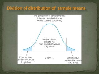
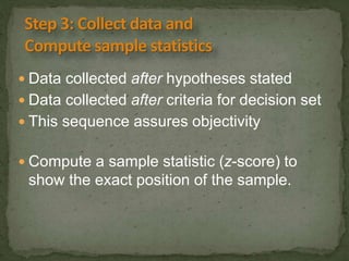
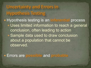
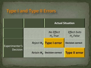
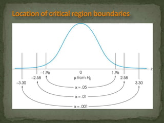
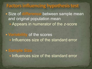
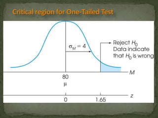
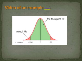
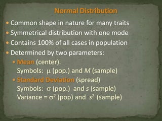
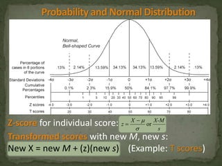
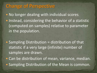
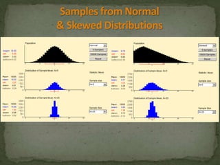
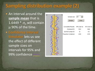
This document provides an overview of key concepts related to the normal distribution, sampling distributions, estimation, and hypothesis testing. It defines important terms like the normal curve, z-scores, sampling distributions, point and interval estimates, and the steps of hypothesis testing including stating hypotheses, collecting data, and determining whether to reject the null hypothesis. It also reviews concepts like the central limit theorem, standard error, bias, confidence intervals, types of errors in hypothesis testing, and factors that influence test statistics.

1. Recap of Normal Distribution
Sampling Distribution
Estimation
Steps of Hypothesis Testing

2.  Normal curve: brief review
 “Standardized scores” brief review
 Z-scores
 Transformed scores (e.g., T-score, IQ, SAT)
 Sampling Distributions
 Estimation: Confidence Intervals
 Hypothesis Testing

3. Areas
Z-scores
Transformed scores (e.g., T-scores)

4.  Common shape in nature for many traits
 Symmetrical distribution with one mode
 Contains 100% of all cases in population
 Determined by two parameters:
 Mean (center).
Symbols:  (pop.) and M (sample)
 Standard Deviation (spread)
Symbols:  (pop.) and s (sample)
Variance = 2 (pop) and s2 (sample)

5. X 
X-M
Z-score for individual score:
z 
or

s
Transformed scores with new M, new s:
New X = new M + (z)(new s) (Example: T scores)

6. X X M
Z-score for individual score:
z
s
Transformed scores with new M, new s:
New X = new M + (z)(new s)
(Examples: T scores, IQ, SAT and GRE, etc.)
 
 or



7. Shape of the distribution
Standard Error

8.  No longer dealing with individual scores
 Instead, considering the behavior of a statistic
(computed on samples) relative to parameter
in the population.
 Sampling Distribution = distribution of that
statistic if a very large (infinite) number of
samples are drawn.
 Can be distribution of mean, variance, median.
 Sampling Distribution of the Mean is common.

11. Bias and
Variability
Simulation
from the
Estimation
Chapter

12.  When many samples are drawn, the
distribution of their means is normal.
 This is true regardless of the shape of the
population’s distribution.
 The Mean of the sampling distribution is equal
to the Population Mean 
2 2
 

2 so or
  

N N N M M

13.  Variance of sampling distribution is equal to
population variance divided by N (sample size)
 Standard deviation of the sampling
distribution is called the “Standard Error”
(of the parameter). It is square root of the
variance of the sampling distribution.
2 2
 

2 so or
  

N N N M M

14. Point Estimates
Interval Estimates

15.  Use our knowledge of sampling distribution to
make a guess about the population when we
only have information from a sample.
 First examples are artificially simple: they give
us the population standard deviation while we
don’t know the population mean.

16.  The mean of the distribution of sample means
is equal to the population mean .
 The mean of the sampling distribution is called
the expected value of the statistic
 The sample mean is an unbiased estimator of
the population mean .

17.  The mean of a single sample is an unbiased
estimator of the population mean 
 The Standard Error of the Mean (when we
know the population standard deviation )
gives us information about the expected
deviation score of our sample mean M from
the population parameter 
We use this information, and the areas of the
normal curve, to compute an interval estimate.

18. M = 30,  = 9, N =25, 90% confidence interval
We find z.90 from the Inverse Normal
Calculator (here) for the Unit Normal Curve
(z = 1.6449 for a 90% confidence interval)
 According to the Central Limit theorem, the
middle 90% of sample means will be within
1.6449 M of the population mean 
 Therefore, the probability that the population
mean will be within 1.6449 M is also 90%

19.  An interval around the
sample mean that is
1.6449 * M will contain
 90% of the time.
 Confidence Interval
Simulator lets us see
the effect of different
sample sizes on
intervals for 95% and
99% confidence (here)

20.  Calculate the Standard Error of the Mean:
M = /N = 9/ 25 = 9/5 = 1.80
 Calculate Confidence Interval by hand:
 Lower limit = M – (1.6449*1.80) = 35-2.96082
 Upper limit = M + (1.6449*1.80) = 35+2.96082
 90% Confidence Interval
= [32.03918, 37.96082 ]

21.  Remember:
M is the Standard
Deviation of the
Sampling
Distribution, so we
will use M in the
Inverse Normal
Calculator.

22. Null hypothesis and Alternate Hypotheses
Reject a Null hypothesis when it is very unlikely

23. 1. State a null hypothesis about a population
2. Predict the characteristics of the sample
based on the hypothesis
3. Obtain a random sample from the population
4. Compare the obtained sample data with the
prediction made from the hypothesis
 If consistent, hypothesis is reasonable
 If discrepant, hypothesis is rejected

24. • Trial begins with null hypothesis
(innocent until proven guilty).
• Police and prosecutor gather evidence (data)
about probable innocence.
• If there is sufficient evidence, jury rejects
innocence claim and concludes guilt.
• If there is not enough evidence, jury fails to
convict (but does not conclude defendant
is innocent).

25.  State the hypotheses
 Null hypothesis or H0
 Alternate hypothesis or HA or H1
 Set the criteria for a decision
 Pick an alpha level (.05 is common)
 Collect data and compute sample statistics
 Need mean and standard deviation
 Make a decision

26.  Null hypothesis (H0) states that, in the
general population, there is no change, no
difference, or no relationship
 Alternative hypothesis (H1) states that
there is a change, a difference, or a
relationship in the general population

27.  Distribution of sample means is divided
 Those likely if H0 is true
 Those very unlikely if H0 is true
 Alpha level, or level of significance, is a
probability value used to define “very unlikely”
 Critical region is composed of the extreme
sample values that are very unlikely
 Boundaries of critical region are determined
by alpha level.

30.  Data collected after hypotheses stated
 Data collected after criteria for decision set
 This sequence assures objectivity
 Compute a sample statistic (z-score) to
show the exact position of the sample.

31.  If sample data are in
the critical region,
the null hypothesis is
rejected
 If the sample data are
not in the critical
region, the researcher
fails to reject the null
hypothesis

32.  Hypothesis testing is an inferential process
 Uses limited information to reach a general
conclusion, often leading to action
 Sample data used to draw conclusion
about a population that cannot be
observed.
 Errors are possible and probable

33. Actual Situation
No Effect
H0 True
Effect Exits
H0 False
Experimenter’s
Decision
Reject H0 Type I error Decision correct
Retain H0 Decision correct Type II error

35.  Size of difference between sample mean
and original population mean
 Appears in numerator of the z-score
 Variability of the scores
 Influences size of the standard error
 Sample Size
 Influences size of the standard error

36.  In a two-tailed test, the critical region is
divided on both tails of the distribution.
 Researchers usually have a specific
prediction about the direction of a
treatment effect before they begin.
 In a directional hypothesis or one-tailed
test, the hypotheses specify an increase or
decrease in the population mean

39. It all makes sense when a teacher walks through it.
The ideas become yours when you work with them.

40. Recap of Normal Distribution
Sampling Distribution
Estimation
Steps of Hypothesis Testing