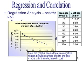
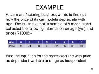
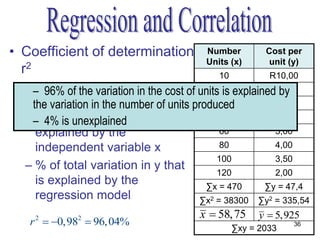
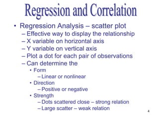
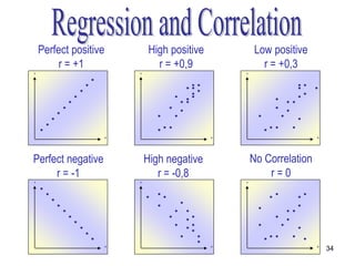
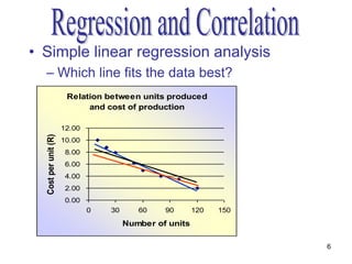
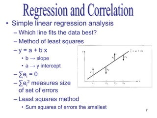
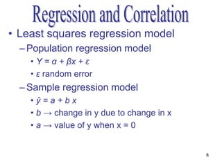
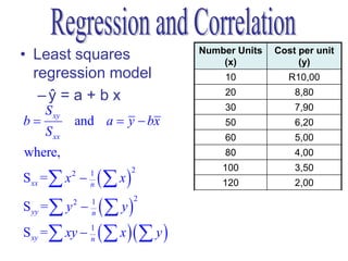
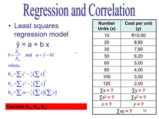
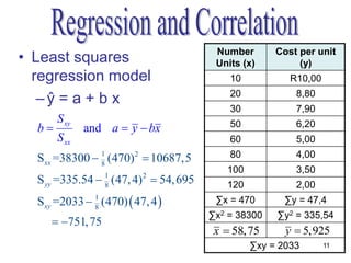
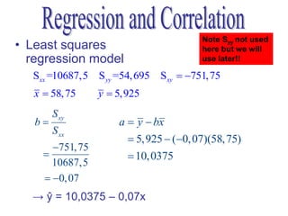
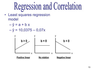
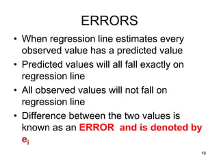
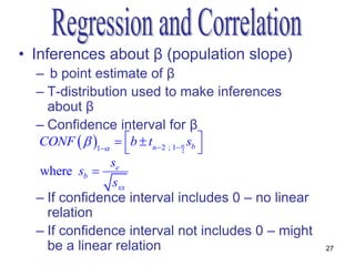
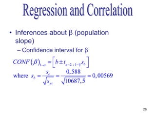
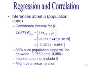
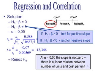
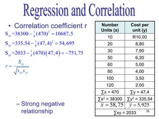
- Regression analysis determines the relationship between two quantitative variables and derives an equation to describe their relationship. - A scatter plot is used to display the relationship between the independent and dependent variables and determine if it is linear or nonlinear. - The method of least squares is used to fit a linear regression line that minimizes the sum of the squared residuals between observed and predicted values of the dependent variable. 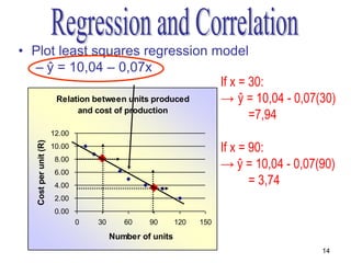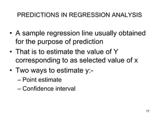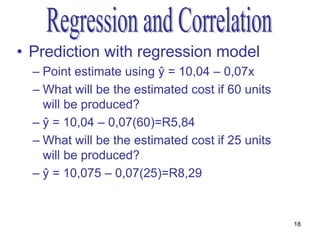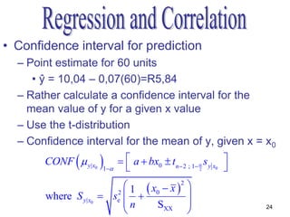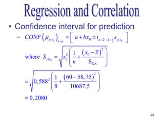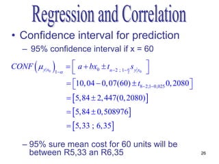- The regression equation can be used to predict values of the dependent variable for given values of the independent variable.

1. 1

2. • Analyze the relationship among two
quantitative variables
• Correlation determines the strength and
direction between the variables
• Regression determines a mathematical
equation to explain the relation
• Equation can be used for prediction
2

3. • Regression Analysis
– X → independent variable
– Y → dependent variable
– Independent variable influence depended variable
– Sample consists of n pairs of observations
– Ascertain if a relation exists
– Examine the nature of the relation
– Obtain an equation that relates Y to X
– The magnitude in change of one variable due to
change in another variable can be evaluated
– Predict value of Y on different values of X
3

4. • Regression Analysis – scatter plot
– Effective way to display the relationship
– X variable on horizontal axis
– Y variable on vertical axis
– Plot a dot for each pair of observations
– Can determine the
• Form
– Linear or nonlinear
• Direction
– Positive or negative
• Strength
– Dots scattered close – strong relation
– Large scatter – weak relation 4

5. • Regression Analysis – scatter Number Cost per
Units (x) unit (y)
plot
10 R10,00
– Example 20 8,80
Relation between units produced
– Two variables production
and cost of 30 7,90
• 12.00 of producing units
Cost 50 6,20
Cost per unit (R)
• 10.00
Number of units produced 60 5,00
8.00
80 4,00
– Cost is depending on number of
6.00
100 3,50
units
4.00
2.00 120 2,00
0.00
0 30 60 90 120 150
From theof unitsit seems there is a negative
Number graph
relation between number of units and cost
– more units then decrease in cost 5

6. • Simple linear regression analysis
– Which line fits the data best?
Relation between units produced
and cost of production
12.00
Cost per unit (R)
10.00
8.00
6.00
4.00
2.00
0.00
0 30 60 90 120 150
Number of units
6

7. • Simple linear regression analysis
– Which line fits the data best?
– Method of least squares
–y=a+bx
• b → slope
• a → y intercept
– ∑ei = 0
– ∑ei2 measures size
of set of errors
– Least squares method
• Sum squares of errors the smallest 7

8. • Least squares regression model
– Population regression model
• Y = α + βx + ε
• ε random error
– Sample regression model
•ŷ=a+bx
• b → change in y due to change in x
• a → value of y when x = 0
8

9. • Least squares Number Units
(x)
Cost per unit
(y)
regression model 10 R10,00
–ŷ = a + b x 20 8,80
S xy 30 7,90
b and a  y  bx 50 6,20
S xx 60 5,00
where, 80 4,00
 x
100 3,50
Sxx =  x  2 1 2
n 120 2,00
 y
∑x = 470 ∑y = 47,4
S yy =  y 2 1 2
n ∑x2 = 38300 ∑y2 = 335,54
Sxy =  xy  1
n   x   y  x  58,75 y  5,925
∑xy = 2033 9

10. Number Cost per unit
• Least squares Units (x) (y)
regression model 10 R10,00
ŷ=a+bx 20 8,80
30 7,90
S xy
b and a  y  bx 50 6,20
S xx
60 5,00
where,
80 4,00
Sxx =  x   x
2 1 2
n 100 3,50
S yy =  y   y
2 1 2
n
120 2,00
Sxy =  xy  1
n   x   y  ∑x = ? ∑y = ?
∑x2 = ? ∑y2 = ?
Calculate Sxx, Syy, Sxy
∑xy = ? 10

11. Number Cost per unit
• Least squares Units (x) (y)
regression model 10 R10,00
–ŷ = a + b x 20 8,80
30 7,90
S xy
b and a  y  bx 50 6,20
S xx 60 5,00
Sxx =38300  1 (470) 2  10687,5
8
80 4,00
100 3,50
S yy =335.54  (47, 4)  54, 695
1
8
2
120 2,00
Sxy =2033  1 (470)  47, 4 
8
∑x = 470 ∑y = 47,4
∑x2 = 38300 ∑y2 = 335,54
 751, 75
x  58,75 y  5,925
∑xy = 2033 11

12. Note Syy not used
• Least squares here but we will
regression model use later!!
Sxx =10687,5 S yy =54, 695 Sxy  751, 75
x  58, 75 y  5,925
S xy
b a  y  bx
S xx
 5,925  (0, 07)(58, 75)
751, 75
  10, 0375
10687,5
 0, 07
→ ŷ = 10,0375 – 0,07x

13. • Least squares regression
model
–ŷ=a+bx
– ŷ = 10,0375 – 0,07x
y y y
b>0 b=0 b<0
x x x
Positive linear No relation Negative linear
13

14. • Plot least squares regression model
– ŷ = 10,04 – 0,07x
If x = 30:
Relation between units produced → ŷ = 10,04 - 0,07(30)
and cost of production
=7,94
12.00
If x = 90:
Cost per unit (R)
10.00
8.00
6.00
→ ŷ = 10,04 - 0,07(90)
4.00 = 3,74
2.00
0.00
0 30 60 90 120 150
Number of units
14

15. EXAMPLE
A car manufacturing business wants to find out
how the price of its car models depreciate with
age. The business took a sample of 8 models and
collected the following information on age (yrs) and
price (R1000):-
Age 8 3 6 9 2 5 6 3
Price 16 74 38 19 102 36 33 69
Find the equation for the regression line with price
as dependent variable and age as independent
15

16. Example answer
Example 11.4, textbook, part 2, page 383
16

17. PREDICTIONS IN REGRESSION ANALYSIS
• A sample regression line usually obtained
for the purpose of prediction
• That is to estimate the value of Y
corresponding to as selected value of x
• Two ways to estimate y:-
– Point estimate
– Confidence interval
17

18. • Prediction with regression model
– Point estimate using ŷ = 10,04 – 0,07x
– What will be the estimated cost if 60 units
will be produced?
– ŷ = 10,04 – 0,07(60)=R5,84
– What will be the estimated cost if 25 units
will be produced?
– ŷ = 10,075 – 0,07(25)=R8,29
18

19. ERRORS
• When regression line estimates every
observed value has a predicted value
• Predicted values will all fall exactly on
regression line
• All observed values will not fall on
regression line
• Difference between the two values is
known as an ERROR and is denoted by
ei
19

20. ERRORS
• Since the observed values deviate from the
predicted values the regression equation is not a
perfect predictor
• Need to be able to assess the accuracy of the
regression line in predicting the values and this
is done by analysing the errors ei
• STD DEV errors measures how widely observed
values are spread around regression line
• The smaller the STD DEV the closer the points
cluster around line
20

21. • Standard deviation
Number Cost Predicted Difference ei
of random errors Units per cost per = yi - ŷi
(x) unit (y) unit (ŷ)
– ŷ = 10,04 – 0,07x 10 10,00 9,34 0,66
ŷ = 10,04 – 0,07(10) = 9,34
– ei indicate how 8,64
0,07(20) the 20 8,80 8,64 0,16
observed and 30 7,90 7,94 -0,04
expected values 50 6,20 6,54 -0,34
differ 60 5,00 5,84 -0,84
– Standard deviation 80 4,00 4,44 -0,44
of errors measures 100 3,50 3,04 0,46
spread around the 120 2,00 1,64 0,36
line
• Smaller - points
closer to line 21

22. • Standard deviation Number
Units
Cost
per
Predicted
cost per
Difference ei
= yi - ŷi
of random errors (x) unit (y) unit (ŷ)
10 10,00 9,34 0,66
S yy  bS xy
Se  20 8,80 8,64 0,16
n2 30 7,90 7,94 -0,04
54, 695  (0, 07)(751, 75) 50 6,20 6,54 -0,34
 60 5,00 5,84 -0,84
82 80 4,00 4,44 -0,44
 0,588 100 3,50 3,04 0,46
– Small 120 2,00 1,64 0,36
– Values close to line
22

23. CONFIDENCE INTERVAL FOR PREDICTION
• Different samples from the same population will
give different point estimates
• Likely that different samples from same
population will give different estimated
regression lines
• Therefore need to construct a confidence
interval for Y based on one sample that will give
a more reliable estimate of Y
• Generally called a PREDICTION INTERVAL
23

24. • Confidence interval for prediction
– Point estimate for 60 units
• ŷ = 10,04 – 0,07(60)=R5,84
– Rather calculate a confidence interval for the
mean value of y for a given x value
– Use the t-distribution
– Confidence interval for the mean of y, given x = x0

CONF  y| x0 1
  a  bx0  tn  2 ; 1  s y x0 
 2 
 1  x0  x 2 
where S y| x0  se2   
n SXX 
  24

25. • Confidence interval for prediction
– CONF   y| x    a  bx0  tn  2 ; 1  s y x0 
0 1  2 
 1  x0  x 2 
where S y| x0  se2   
n SXX 
 
 1  60  58, 75 2 
 0,5882   
8 10687,5 
 
 0, 2080
25

26. • Confidence interval for prediction
– 95% confidence interval if x = 60

CONF  y| x0 
1
  a  bx0  tn  2 ; 1  s y x0 
 2 
 10, 04  0, 07(60)  t8 2;10,025 0, 2080 
 
 5,84  2, 447(0, 2080) 
 5,84  0,508976
 5,33 ; 6,35
– 95% sure mean cost for 60 units will be
between R5,33 an R6,35 26

27. • Inferences about β (population slope)
– b point estimate of β
– T-distribution used to make inferences
about β
– Confidence interval for β
CONF   1  b  tn  2 ; 1  sb 
 2 
se
where sb 
sxx
– If confidence interval includes 0 – no linear
relation
– If confidence interval not includes 0 – might
be a linear relation 27

28. • Inferences about β (population
slope)
– Confidence interval for β
CONF   1  b  tn  2 ; 1  sb 
 2 
se 0,588
where sb    0, 00569
sxx 10687,5
28

29. • Inferences about β (population
slope)
– Confidence interval for β
CONF   1  b  tn  2 ; 1  sb 
 2 
  0, 07  2, 447(0, 00569
  0, 0839 ;  0, 0561
– 95% sure population slope will be
between -0,0839 and -0,0561
– Interval does not include 0
– Might be a linear relation 29

30. • Inferences about β (population slope)
– Hypothesis test concerning β
Testing H0: β = 0 for n < 30
Alternative Decision rule:
Test statistic
hypothesis Reject H0 if
H1: β ≠ 0 |t| ≥ tn - 2;1- α/2 t
b
sb
H1: β > 0 t ≥ tn-2;1- α
se
with sb 
H1: β < 0 t ≤ -tn-2;1- α sxx
30

31. • Solution -2,447 +2,447
– H0 : β = 0 Reject H0 Accept H0 Reject H0
– H1 : β ≠ 0
– α = 0,05
If H1 : β > 0 - test for positive slope
se 0,588
sb   0, 00569β < 0 - test for negative slope
sxx 10687,5 If H1 :
b 0, 07
 
t–  12,346
sb 0, 00569
At α = 0,05 the slope is not zero –
– Reject H0
there is a linear relation between
number of units and cost per unit 31

32. • Correlation Analysis
– Strength of linear relationship
– Direction of linear relationship
• Positive
• Negative
– Population correlation coefficient ρ (rho)
– Sample correlation coefficient r
– r always between -1 and +1
• r = 1 perfect positive
• r = -1 perfect negative
• r = 0 no relationship
• near 0 weak relationship
• near -1 or +1 strong relationship 32

33. Coefficient of correlation
• The coefficient of correlation is used to measure
the strength of association between two
variables.
• The coefficient values range between -1 and 1.
– If r = -1 (negative association) or r = +1
(positive association) every point falls on the
regression line.
– If r = 0 there is no linear pattern.
• The coefficient can be used to test for linear
relationship between two variables. 33

34. Perfect positive High positive Low positive
r = +1 r = +0,9 r = +0,3
Y Y Y
X X X
Perfect negative High negative No Correlation
r = -1 r = -0,8 r=0
Y Y Y
X X X
34

35. • Correlation coefficient r Number
Units (x)
Cost per
unit (y)
Sxx =38300  1 (470) 2  10687,5
8 10 R10,00
S yy =335.54  1 (47, 4) 2  54, 695
8 20 8,80
Sxy =2033  1 (470)  47, 4   751, 75
8
30 7,90
50 6,20
S xy
r 60 5,00
sxx s yy 80 4,00
751, 75 100 3,50
 120 2,00
10687,5(54, 695)
∑x = 470 ∑y = 47,4
 0,98 ∑x2 = 38300 ∑y2 = 335,54
– Strong negative x  58,75 y  5,925
relationship ∑xy = 2033 35

36. • Coefficient of determination Number Cost per
Units (x) unit (y)
r2 10 R10,00
– – 96% of the proportionthe cost of units20 explained8,80
Measures variation in of is by
the variation inthe number of units produced
changes in the dependent 30 7,90
– 4% is unexplained be
variable y that can 50 6,20
explained by the 60 5,00
independent variable x 80 4,00
100 3,50
– % of total variation in y that
120 2,00
is explained by the ∑x = 470 ∑y = 47,4
regression model ∑x2 = 38300 ∑y2 = 335,54
x  58,75 y  5,925
r  0,98  96,04%
2 2
36
∑xy = 2033

37. • Hypothesis test concerning the
correlation coefficient ρ
Testing H0: ρ = 0 for n < 30
Alternative Decision rule:
Test statistic
hypothesis Reject H0 if
r
t
H1: ρ ≠ 0 |t| ≥ tn - 2;1- α/2 1 r2
n2
37

38. • Solution -2,447 +2,447
– H0 : ρ = 0 Reject H0 Accept H0 Reject H0
– H1 : ρ ≠ 0
– α = 0,05
r 0,98
t   12, 06
1 r2 1  (0,98) 2
– n2 82
At α = 0,05 the correlation coefficient is
– Reject H0 not zero – there is a linear relation
between number of units and cost per unit 38