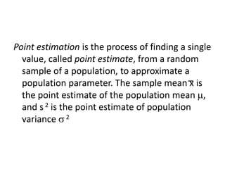
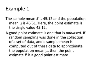
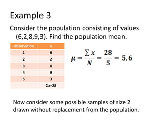
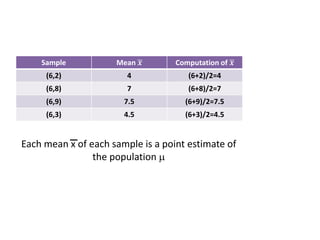
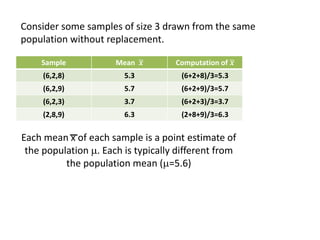
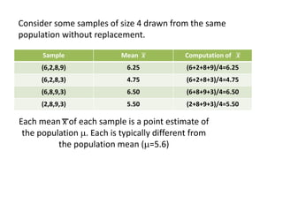
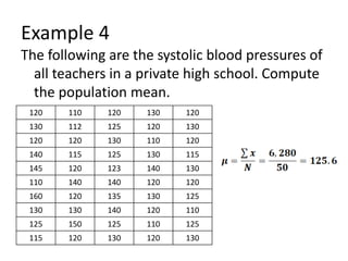
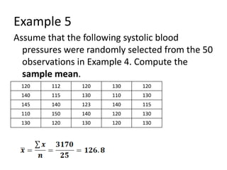
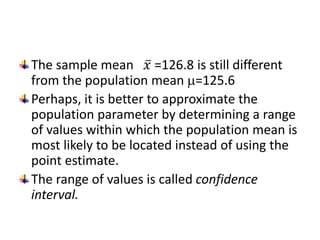
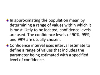
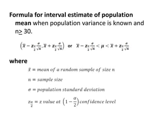
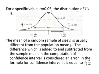
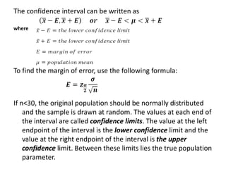
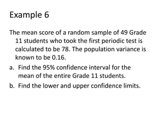
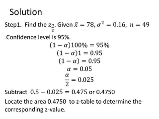
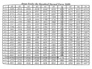
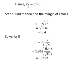
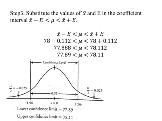
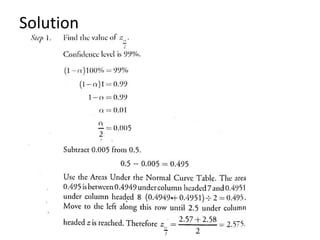
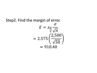
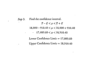
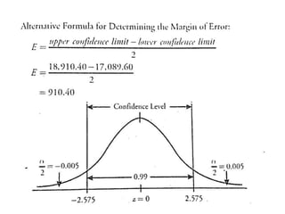
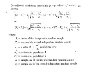
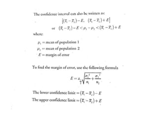
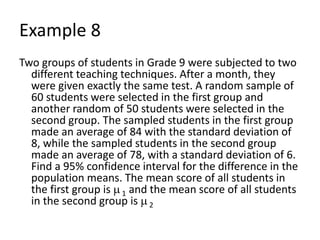
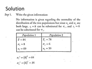
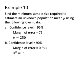
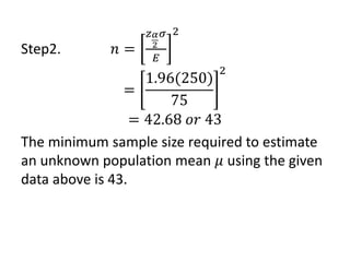
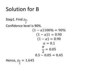
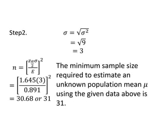
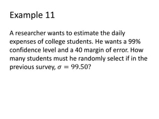
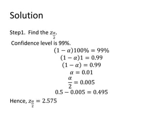
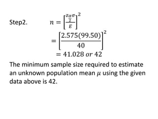
6. point and interval estimation

Learning Competencies
The learner will be able to:
1. Illustrate point and interval estimations;
2. Distinguish between point and interval estimation;
3. Identify point estimator for the population mean;
4. Compute for the point estimate for the population
mean;
5. Identify the appropriate form of the confidence
interval estimator for the population mean when
the population variance is known; and
6. Compute for the confidence interval estimate based
on the appropriate form of the estimator for the
population mean.

Point estimation is the process of finding a single
value, called point estimate, from a random
sample of a population, to approximate a
population parameter. The sample mean x is
the point estimate of the population mean ,
and s 2 is the point estimate of population
variance 2

Example 1
The sample mean 𝑥 is 45.12 and the population
mean  is 46.51. Here, the point estimate is
the single value 45.12.
A good point estimate is one that is unbiased. If
random sampling was done in the collection
of a set of data, and a sample mean is
computed out of these data to approximate
the population mean , then the point
estimate 𝑥 is a good point estimate.

Example 2
A teacher wanted to determine the average
height of Grade 9 students in their school.
What he did was to go to the one of the eight
sections in Grade 9 and then took their
heights. He computed for the mean height of
the students and got 165 cm.

Here, 165 cm is not a good point estimate of the
population mean. The teacher should have
randomly selected the members of his sample
from the entire population using either a
simple random sampling or systematic
random sampling.

A researcher should not expect the point
estimate to be exactly equal to the population
parameter. However, any point estimate used
should be as close as possible to the true
parameter.
Data should be carefully collected.
Sampling should be done at random, and the
sample size should be large especially when
the population distribution is not normal.
Different samples of size n taken from the
same population produce different results.

In the case of a sample mean 𝑥, the result is
affected by the presence of outliers. These are
data that are numerically too far from the rest
of the data.

Example 3
Consider the population consisting of values
(6,2,8,9,3). Find the population mean.
Observation x
1 6
2 2
3 8
4 9
5 3
x=28
Now consider some possible samples of size 2
drawn without replacement from the population.

Sample Mean 𝒙 Computation of 𝒙
(6,2) 4 (6+2)/2=4
(6,8) 7 (6+8)/2=7
(6,9) 7.5 (6+9)/2=7.5
(6,3) 4.5 (6+3)/2=4.5
Each mean x of each sample is a point estimate of
the population 

(6,2,8) 5.3 (6+2+8)/3=5.3
(6,2,9) 5.7 (6+2+9)/3=5.7
(6,2,3) 3.7 (6+2+3)/3=3.7
(2,8,9) 6.3 (2+8+9)/3=6.3
the population . Each is typically different from
the population mean (=5.6)
Consider some samples of size 3 drawn from the same
population without replacement.

(6,2,8,9) 6.25 (6+2+8+9)/4=6.25
(6,2,8,3) 4.75 (6+2+8+3)/4=4.75
(6,8,9,3) 6.50 (6+8+9+3)/4=6.50
(2,8,9,3) 5.50 (2+8+9+3)/4=5.50
the population . Each is typically different from
the population mean (=5.6)
Consider some samples of size 4 drawn from the same
population without replacement.

Example 4
The following are the systolic blood pressures of
all teachers in a private high school. Compute
the population mean.
120 110 120 130 120
130 112 125 120 130
120 120 130 110 120
140 115 125 130 115
145 120 123 140 130
110 140 140 120 120
160 120 135 130 125
130 130 140 120 110
125 150 125 110 125
115 120 130 120 130

Example 5
Assume that the following systolic blood
pressures were randomly selected from the 50
observations in Example 4. Compute the
sample mean.
120 112 120 130 120
140 115 130 110 130
145 140 123 140 115
110 150 140 120 130
130 120 130 120 130

The sample mean 𝑥 =126.8 is still different
from the population mean =125.6
Perhaps, it is better to approximate the
population parameter by determining a range
of values within which the population mean is
most likely to be located instead of using the
point estimate.
The range of values is called confidence
interval.

In approximating the population mean by
determining a range of values within which it
is most likely to be located, confidence levels
are used. The confidence levels of 90%, 95%,
and 99% are usually chosen.
Confidence interval uses interval estimate to
define a range of values that includes the
parameter being estimated with a specified
level of confidence.

Confidence level refers to the probability that
the confidence interval contains the true
population parameter. Its value is
confidence level=(1-)100%,
where =probability that the confidence
interval does not contain the true population
parameter.

The value of alpha  corresponds to the level
of significance. The value of alpha  can be
arbitrarily chosen. Any number between 0 and
1 can be used for alpha  but 0.10, 0.05, and
0.01 are the ones that are commonly used.
A 95% confidence level implies that the
probability of the confidence interval
containing the true population parameter is
95%.

Critical value is the value that indicates the
point beyond which lies the rejection region.
This region does not contain the true
population parameter.

INTERVAL ESTIMATE
OF POPULATION
MEAN WITH KNOWN
VARIANCE

Formula for interval estimate of population
mean when population variance is known and
n> 30.
where

For a specific value, =0.05, the distribution of x’s
is:
The mean of a random sample of size n is usually
different from the population mean . The
difference which is added to and subtracted from
the sample mean in the computation of
confidence interval is considered an error. In the
formula for confidence interval it is equal to

The confidence interval can be written as
where
To find the margin of error, use the following formula:
If n<30, the original population should be normally distributed
and the sample is drawn at random. The values at each end of
the interval are called confidence limits. The value at the left
endpoint of the interval is the lower confidence limit and the
value at the right endpoint of the interval is the upper
confidence limit. Between these limits lies the true population
parameter.

Example 6
The mean score of a random sample of 49 Grade
11 students who took the first periodic test is
calculated to be 78. The population variance is
known to be 0.16.
a. Find the 95% confidence interval for the
mean of the entire Grade 11 students.
b. Find the lower and upper confidence limits.

Solution
Step1. Find the 𝑧𝛼
2
. Given 𝑥 = 78, 𝜎2
= 0.16, 𝑛 = 49
Confidence level is 95%.
1 − 𝛼 100% = 95%
1 − 𝛼 1 = 0.95
1 − 𝛼 = 0.95
𝛼 = 0.05
𝛼
2
= 0.025
Subtract 0.5 − 0.025 = 0.475 or 0.4750
Locate the area 0.4750 to z-table to determine the
corresponding z-value.

Hence, 𝑧𝛼
2
= 1.96
Step2. Find 𝜎, then find the margin of error E.
𝜎 = 𝜎2
= 0.16
= 0.4
Solve for E
𝐸 = 𝑧𝛼
2
𝜎
𝑛
= 1.96
0.4
49
= 0.112

Step3. Substitute the values of 𝑥 and E in the coefficient
interval 𝑥 − 𝐸 < 𝜇 < 𝑥 + 𝐸.
𝑥 − 𝐸 < 𝜇 < 𝑥 + 𝐸
78 − 0.112 < 𝜇 < 78 + 0.112
77.888 < 𝜇 < 78.112
77.89 < 𝜇 < 78.11

Conclusion:
The researcher is 95% confident that the sample
mean 78 differs from the population mean by
no more than 0.112 or 0.11. Also, the
researcher is 95% confident that the
population mean is between 77.89 and 78.11
when the mean of the sample is 78.

Example 7
Assuming normality, use the given confidence level
and sample data below to find the following:
a. Margin of error
b. Confidence interval for estimating the
population parameter
Given data:
99% confidence level
n=50
x=18,000
=2,500

Step2. Find the margin of error.
𝐸 = 𝑧𝛼
2
𝜎
𝑛
= 2.575
2,500
50
= 910.40

Conclusion:
The researcher is 99% confident that the sample
mean 18,000 differs from the population
mean by no more than 910.40. The value of
the population mean is within the interval
17,089.60 and 18,910.40.

ESTIMATING THE
DIFFERENCE BETWEEN
TWO POPULATION
MEANS

The point estimate for the difference of two
populations means To obtain
this point estimate, select two independent
random samples, one from each population
with sizes n1 and n2, then, compute the
difference between their means.

Example 8
Two groups of students in Grade 9 were subjected to two
different teaching techniques. After a month, they
were given exactly the same test. A random sample of
60 students were selected in the first group and
another random of 50 students were selected in the
second group. The sampled students in the first group
made an average of 84 with the standard deviation of
8, while the sampled students in the second group
made an average of 78, with a standard deviation of 6.
Find a 95% confidence interval for the difference in the
population means. The mean score of all students in
the first group is 1 and the mean score of all students
in the second group is 2

Step2. Find the value of 𝑧𝛼
2
. Confidence level is 95%.
1 − 𝛼 100% = 95%
1 − 𝛼 = 0.95
𝛼 = 0.05
𝛼
2
=
0.05
2
= 0.025
0.500 − 0.025 = 0.475
Using the areas under the normal curve table, 𝑧𝛼
2
=
1.96

Example 9
Independent random samples were selected
from two populations. The sample means,
known population variance, and sample sizes
are given in the following table:
Find a 90% confidence interval for estimating
the difference in the population means
𝜇1 − 𝜇2 .
Population 1 Population 2
Sample mean 34 38
Population variance 5 7
Sample size 40 46

Solution
Step1. Write the given information
Step2. Find the value of 𝑧𝛼
2
. Confidence level is 90%.
Population 1 Population 2
𝑥1 = 34 𝑥2 = 38
𝜎1
2 = 5 𝜎2
2 = 7
𝑛1 = 40 𝑛2 = 46
1 − 𝛼 100% = 90%
1 − 𝛼 = 0.90
𝛼 = 0.1
𝛼
2
=
0.1
2
= 0.05
0.500 − 0.05 = 0.45
The area to the right of 𝑧𝛼
2
is
0.05.
The area to the left of 𝑧𝛼
2
is 0.05.
From the areas under the
normal curve table, 𝑧𝛼
2
= 1.645

Step3. Find the margin of error.
𝐸 = 𝑧𝛼
2
𝜎1
2
𝑛1
+
𝜎2
2
𝑛2
= 1.645
5
40
+
7
46
= 0.866 𝑜𝑟 0.87

Step4. Find the confidence interval
𝑥1 − 𝑥2 − 𝐸 < 𝝁𝟏 − 𝝁𝟐 < 𝑥1 − 𝑥2 + 𝐸
34 − 38 − 0.87 < 𝝁𝟏 − 𝝁𝟐 < 34 − 38 + 0.87
−4 − 0.87 < 𝝁𝟏 − 𝝁𝟐 < −4 + 0.87
−4.87 < 𝝁𝟏 − 𝝁𝟐 < −3.13
It is possible that the difference between the two
population means 𝜇1 − 𝜇2 could be negative. This
indicates that the mean of population 1 could be
less than that of population 2.

SAMPLE SIZE FOR
ESTIMATING
POPULATION MEAN 𝝁

The size of the sample is important in estimating the
population mean 𝜇. The following formula can be used to
determine the appropriate sample size.
Sample size for Estimating 𝝁:
𝒏 =
𝒛𝜶
𝟐
𝝈
𝑬
𝟐
where 𝑧𝛼
2
=
𝑐𝑟𝑖𝑡𝑖𝑐𝑎𝑙 𝑣𝑎𝑙𝑢𝑒 𝑏𝑎𝑠𝑒𝑑 𝑜𝑛 𝑡ℎ𝑒 𝑑𝑒𝑠𝑖𝑟𝑒𝑑 𝑐𝑜𝑛𝑓𝑖𝑑𝑒𝑛𝑐𝑒 𝑙𝑒𝑣𝑒𝑙
𝐸 = 𝑑𝑒𝑠𝑖𝑟𝑒𝑑 𝑚𝑎𝑟𝑔𝑖𝑛 𝑜𝑓 𝑒𝑟𝑟𝑜𝑟
𝜎 = 𝑝𝑜𝑝𝑢𝑙𝑎𝑡𝑖𝑜𝑛 𝑠𝑡𝑎𝑛𝑑𝑎𝑟𝑑 𝑑𝑒𝑣𝑖𝑎𝑡𝑖𝑜𝑛

Example 10
Find the minimum sample size required to
estimate an unknown population mean 𝜇 using
the following given data.
a. Confidence level = 95%
Margin of error = 75
𝜎 = 250
b. Confidence level = 90%
Margin of error = 0.891
𝜎2
= 9

Solution for A
Step1. Find 𝑧𝛼
2
.
1 − 𝛼 100% = 95%
1 − 𝛼 1 = 0.95
1 − 𝛼 = 0.95
𝛼 = 0.05
𝛼
2
= 0.025
0.5 − 0.025 = 0.475
Hence, 𝑧𝛼
2
= 1.96

Step2. 𝑛 =
𝑧𝛼
2
𝜎
𝐸
2
=
1.96(250)
75
2
= 42.68 𝑜𝑟 43
The minimum sample size required to estimate
an unknown population mean 𝜇 using the given
data above is 43.

Solution for B
Step1. Find 𝑧𝛼
2
.
1 − 𝛼 100% = 90%
1 − 𝛼 1 = 0.90
1 − 𝛼 = 0.90
𝛼 = 0.1
𝛼
2
= 0.05
0.5 − 0.05 = 0.45
Hence, 𝑧𝛼
2
= 1.645

Step2. 𝜎 = 𝜎2
= 9
= 3
𝑛 =
𝑧𝛼
2
𝜎
𝐸
2
=
1.645(3)
0.891
2
= 30.68 𝑜𝑟 31
The minimum sample size
required to estimate an
unknown population mean 𝜇
using the given data above is
31.

Example 11
A researcher wants to estimate the daily
expenses of college students. He wants a 99%
confidence level and a 40 margin of error. How
many students must he randomly select if in the
previous survey, 𝜎 = 99.50?

Solution
Step1. Find the 𝑧𝛼
2
.
1 − 𝛼 100% = 99%
1 − 𝛼 1 = 0.99
1 − 𝛼 = 0.99
𝛼 = 0.01
𝛼
2
= 0.005
0.5 − 0.005 = 0.495
Hence, 𝑧𝛼
2
= 2.575

Step2. 𝑛 =
𝑧𝛼
2
𝜎
𝐸
2
=
2.575(99.50)
40
2
= 41.028 𝑜𝑟 42
The minimum sample size required to estimate
an unknown population mean 𝜇 using the given
data above is 42.

6. point and interval estimation

More Related Content

What's hot

Similar to 6. point and interval estimation

More from ONE Virtual Services

Recently uploaded

In this document

6. point and interval estimation