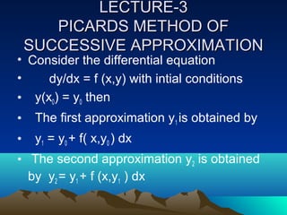
This document provides an overview of numerical methods for solving ordinary differential equations. It outlines several numerical methods including Taylor's series method, Picard's method of successive approximation, Euler's method, modified Euler's method, Runge-Kutta methods, and predictor-corrector methods like Milne's method and Adams-Moulton method. Examples of the formulas used in each method are given. The document also lists references and provides context about the course and unit.

1. UNIT – VI
NUMERICAL SOLUTION OF
ORDINARY DIFFERENTIAL
EQUATIONS

2. MATHEMATICAL METHODS

3. CONTENTS
• Matrices and Linear systems of equations
• Eigen values and eigen vectors
• Real and complex matrices and Quadratic forms
• Algebraic equations transcendental equations and
Interpolation
• Curve Fitting, numerical differentiation & integration
• Numerical differentiation of O.D.E
• Fourier series and Fourier transforms
• Partial differential equation and Z-transforms

4. TEXT BOOKS
• 1.Mathematical Methods, T.K.V.Iyengar, B.Krishna
Gandhi and others, S.Chand and company
• Mathematical Methods, C.Sankaraiah, V.G.S.Book
links.
• A text book of Mathametical Methods,
V.Ravindranath, A.Vijayalakshmi, Himalaya
Publishers.
• A text book of Mathametical Methods, Shahnaz
Bathul, Right Publishers.

5. REFERENCES
• 1. A text book of Engineering Mathematics,
B.V.Ramana, Tata Mc Graw Hill.
• 2.Advanced Engineering Mathematics, Irvin Kreyszig
Wiley India Pvt Ltd.
• 3. Numerical Methods for scientific and Engineering
computation, M.K.Jain, S.R.K.Iyengar and R.K.Jain,
New Age International Publishers
• Elementary Numerical Analysis, Aitkison and Han,
Wiley India, 3rd Edition, 2006.

6. UNIT HEADER
Name of the Course:B.Tech
Code No:07A1BS02
Year/Branch:I Year
CSE,IT,ECE,EEE,ME,CIVIL,AERO
Unit No: VI
No.of slides:32

7. UNIT INDEX
UNIT-VI
S.No. Module Lecture PPT Slide
No. No.
1 Introduction,Taylor’s, L1-3 8-12
Picard’s method.
2 Euler’s, Modified L4-7 13-17
Euler’s R-K Method
3 Milne’s and Adam’s L8-10 18-32
MoultonMethod.

8. LECTURE-1
INTRODUCTION
• There exists large number of ordinary
differential equations, whose solution
cannot be obtained by the known
analytical methods. In such cases, we use
numerical methods to get an approximate
solution o f a given differential equation
with given initial condition.

9. NUMERICAL DIFFERIATION
• Consider an ordinary differential equation of first
order and first degree of the form
• dy/dx = f ( x,y ) ………(1)
• with the intial condition y (x0 ) = y0 which is called
initial value problem.
• T0 find the solution of the initial value
problem of the form (1) by numerical methods,
we divide the interval (a,b) on whcich the
solution is derived in finite number of sub-
intervals by the points

10. LECTURE-2
TAYLOR’S SERIES METHOD
• Consider the first order differential equation
• dy/dx = f ( x, y )……..(1)
with initial conditions y (xo ) = y0 then expanding
y (x ) i.e f(x) in a Taylor’s series at the point xo we
get
y ( xo + h ) = y (x0 ) + hy1(x0) + h2/ 2! Y11(x0)+…….
Note : Taylor’s series method can be applied only
when the various derivatives of f(x,y) exist and
the value of f (x-x0) in the expansion of y = f(x)
near x0 must be very small so that the series is
convergent.

11. LECTURE-3
PICARDS METHOD OF
SUCCESSIVE APPROXIMATION
• Consider the differential equation
• dy/dx = f (x,y) with intial conditions
• y(x0) = y0 then
• The first approximation y1 is obtained by
• y1 = y0 + f( x,y0 ) dx
• The second approximation y2 is obtained
by y2 = y1 + f (x,y1 ) dx

12. PICARDS APPROXIMATION
METHOD
• The third approximation of y3 is obtained y by y2
is given by
• y3 = y0 + f(x,y2) dx……….and so on
• …………………………………
• ………………………………….
• yn = y0 + f (x,yn-1) dx
• The process of iteration is stopped when any
two values of iteration are approximately the
same.
• Note : When x is large , the convergence is slow.

13. LECTURE-4
EULER’S METHOD
• Consider the differential equation
• dy/dx = f(x,y)………..(1)
• With the initial conditions y(x0) = y0
• The first approximation of y1 is given by
• y1 = y0 +h f (x0,,y0 )
• The second approximation of y2 is given
by
• y2 = y1 + h f ( x0 + h,y1)

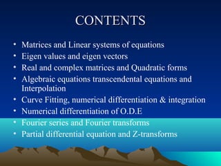
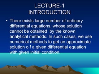
14. EULER’S METHOD
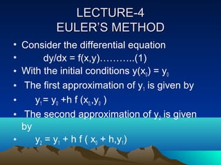
• The third approximation of y3 is given by
• y3 = y2 + h f ( x0 + 2h,y2 )
• ………………………………
• ……………………………..
• ……………………………...
• yn = yn-1 + h f [ x0 + (n-1)h,yn-1 ]
• This is Eulers method to find an appproximate
solution of the given differential equation.

15. IMPORTANT NOTE
• Note : In Euler’s method, we approximate
the curve of solution by the tangent in
each interval i.e by a sequence of short
lines. Unless h is small there will be large
error in yn . The sequence of lines may
also deviate considerably from the curve
of solution. The process is very slow and
the value of h must be smaller to obtain
accuracy reasonably.

16. LECTURE-5
MODIFIED EULER’S METHOD
• By using Euler’s method, first we have to
find the value of y1 = y0 + hf(x0 , y0)
• WORKING RULE
• Modified Euler’s formula is given by
• yik+1 = yk + h/2 [ f(xk ,yk) + f(xk+1,yk+1
• when i=1,y(0)k+1 can be calculated
• from Euler’s method.

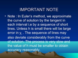
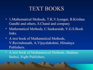
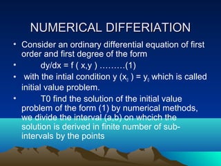
17. MODIFIED EULER’S METHOD
• When k=o,1,2,3,……..gives number of
iterations
• i = 1,2,3,…….gives number of times a
particular iteration k is repeated when
• i=1
• Y1k+1= yk + h/2 [ f(xk,yk) + f(xk+1,y k+1)],,,,,,

18. LECTURE-6
RUNGE-KUTTA METHOD
The basic advantage of using the Taylor series
method lies in the calculation of higher order
total derivatives of y. Euler’s method requires the
smallness of h for attaining reasonable
accuracy. In order to overcomes these
disadvantages, the Runge-Kutta methods are
designed to obtain greater accuracy and at the
same time to avoid the need for calculating
higher order derivatives.The advantage of these
methods is that the functional values only
required at some selected points on the
subinterval.

19. R-K METHOD
• Consider the differential equation
• dy/dx = f ( x, y )
• With the initial conditions y (xo) = y0
• First order R-K method :
• y1= y (x0 + h )
• Expanding by Taylor’s series
• y1 = y0 +h y10 + h2/2 y110 +…….

20. LECTURE-7
R-K METHOD
• Also by Euler’s method
• y1 = y0 + h f (x0 ,y0)
• = y0 + h y10
• It follows that the Euler’s method agrees
with the Taylor’s series solution upto the
term in h. Hence, Euler’s method is the
Runge-Kutta method of the first order.

21. •
• The second order R-K method is given by
• y1= y0 + ½ ( k1 + k2 )
• where k1 = h f ( x0,, y0 )
• k2 = h f (x0 + h ,y0 + k1 )

22. •
• Third order R-K method is given by
• y1 = y0 + 1/6 ( k1 + k2+ k3 )
• where k1 = h f ( x0 , y0 )
• k2 = hf(x0 +1/2h , y0 + ½ k1 )
• k3 =hf(x0 + ½h , y0 + ½ k2)

23. The Fourth order R – K method :
This method is most commonly used and is
often referred to as Runge – Kutta method
only. Proceeding as mentioned above with
local discretisation error in this method
being O (h5), the increment K of y
correspoding to an increment h of x by
Runge – Kutta method from
dy/dx = f(x,y),y(x0)=Y0 is given by

24. •
• K1 = h f ( x 0 , y0 )
• k2 = h f ( x0 + ½ h, y0 + ½ k1 )
• k3 = h f ( x0 + ½ h, y0 + ½ k2 )
• k4 = h f ( x0 + ½ h, y0 + ½ k3 )
• and finally computing
• k = 1/6 ( k1 +2 k2 +2 k3 +k4 )
• Which gives the required approximate value
as
• y1 = y0 + k

25. R-K METHOD
Note 1 : k is known as weighted mean of
k1, k2, k3 and k4.
Note 2 : The advantage of these methods is
that the operation is identical whether the
differential equation is linear or non-linear.

26. LECTURE-8
PREDICTOR-CORRECTOR
METHODS
• We have discussed so far the methods in which
a differential equation over an interval can be
solved if the value of y only is known at the
beginning of the interval. But, in the Predictor-
Corrector method, four prior values are needed
for finding the value of y at xk.
• The advantage of these methods is to estimate
error from successive approximations to yk

27. PREDICTOR-CORRECTOR
METHOD
• If xk and xk+1 be two consecutive points,
such that xk+1=xk+h, then
• Euler’s method is
• Yk+1 = yk + hf(x0 +kh,yk) ,k= 0,1,2,3…….
• First we estimate yk+1 and then this value
of yk+1 is substituted to get a better
approximation of y k+1.

28. LECTURE-9
MILNE’S METHOD
• This procedure is repeated till two consecutive
iterated values of yk+1 are approximately equal.
This technique of refining an initially crude
estimate of yk+1 by means of a more accurate
formula is known as Predictor- Corrector
method.
• Therefore, the equation is called the Predictor
while the equation serves as a corrector of
yk+1.Two such methods, namely, Adams-
Moulton and Milne’s method are discussed.

29. MILNE’S METHOD
• Consider the differntial equation
• dy/dx = f ( x, y ), f (0 ) = 0
• Milne’s predictor formula is given by
• Y(p)n+1=yn-3+4h/3(2y1n-y1n-1+2y1n-2)
• Error estimates
• E (p) = 28/29h5 yv

30. MILNE’S METHOD
• The Milnes corrector formula is givenby
• y(c)n+1=yn-1+h/3(y1n+1+4y1n+y1n-1)
• The superscript c indicates that the
value obtained is the corrected value and
the superscript p on the right indicates that
the predicted value of yn+1 should be used
for computing the value of
• f ( xn+1 , yn+1 ).

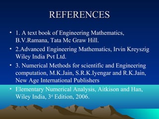
31. LECTURE-10
ADAMS – MOULTON METHOD
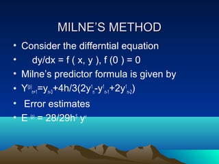
• Consider the differential equation
• dy/dx = f ( x,y ), y(x0) = y0
• The Adams Moulton predictor formula is
given by
• y(p)n+1 = yn + h/24 [55y1n-59y1n-1+37y1n-2- 9y1n-3]

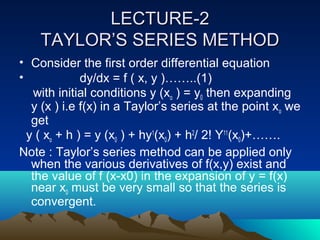
32. ADAM’S MOULTON METHOD
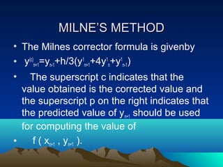
• Adams – Moulton corrector formula is
given by
• Yn+1=yn+h/24[9y1pn+1 +19y1n-5-y1n-1+y1n-2]
Error estimates
EAB = 251/720 h5