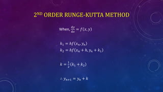
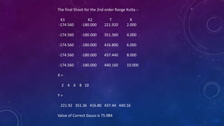
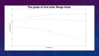
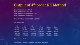
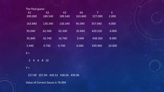
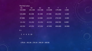
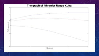
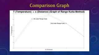
The document outlines a mini project for numerical methods involving the modeling of a heated rod using the Poisson equation and the comparison of temperature distribution solutions obtained from second and fourth order Runge-Kutta methods. It includes a detailed explanation of the shooting method used to solve boundary value problems, along with corresponding data for the iterative solutions and the final outputs for each method. The project showcases graphs comparing the numerical solutions derived from both methods, highlighting the findings and contributions of the group members.

1. 2ME01: NUMERICAL
METHODS AND ANALYSIS
MINI PROJECT (3RD SEMESTER)
QUESTION: 2ME01P.2
GROUP: 7G10

2. PROJECT QUESTION
2ME01P.2. A heated rod with a uniform heat source can be modelled with the
Poisson equation,
ⅆ2 𝑇
ⅆ𝑡2
= −𝑓 𝑥
Given a heat source 𝑓 𝑥 = 0.12𝑥3 − 2.4𝑥2 + 12𝑥 and the boundary conditions,
T(x = 0) = 40 and T(x = 10) = 200, solve for the temperature distribution with the
Range-kutta second and fourth order shooting method (Δ𝑥 = 2). Compare the
numerical solution of each method with the help of graph.

3. ORDINARY DIFFERENTIAL EQUATION
An ordinary differential equation (ODE) is an equality involving a function and its derivatives.
An ODE of order n is an equation of the form
𝑓 𝑥, 𝑦, 𝑦1
, … , 𝑦 𝑛
= 0
where y is a function of x
𝑦1
=
ⅆ𝑦
ⅆ𝑥
is the first derivative with respect to x
.
.
.
𝑦 𝑛 =
ⅆ 𝑛 𝑦
ⅆ𝑥 𝑛 is the nth derivative with respect to x.

4. 2ND ORDER RUNGE-KUTTA METHOD
When,
ⅆ𝑦
ⅆ𝑥
= 𝑓 𝑥, 𝑦
𝑘1 = ℎ𝑓 𝑥 𝑛, 𝑦𝑛
𝑘2 = ℎ𝑓 𝑥 𝑛 + ℎ, 𝑦𝑛 + 𝑘1
𝑘 =
1
2
𝑘1 + 𝑘2
∴ 𝑦 𝑛+1 = 𝑦𝑛 + 𝑘

5. 4TH ORDER RUNGE-KUTTA METHOD
When,
ⅆ𝑦
ⅆ𝑥
= 𝑓 𝑥, 𝑦
𝑘1 = ℎ𝑓 𝑥 𝑛, 𝑦𝑛
𝑘2 = ℎ𝑓 𝑥 𝑛 +
ℎ
2
, 𝑦𝑛 +
𝑘1
2
𝑘3 = ℎ𝑓 𝑥 𝑛 +
ℎ
2
, 𝑦𝑛 +
𝑘2
2
𝑘4 = ℎ𝑓 𝑥 𝑛 + ℎ, 𝑦𝑛 + 𝑘3
𝑘 =
1
6
𝑘1 + 2𝑘2 + 2𝑘3 + 𝑘4
∴ 𝑦 𝑛+1 = 𝑦𝑛 + 𝑘

6. • The shooting method is based on converting the boundary-
value problem into an equivalent initial-value problem. A trial-
and-error approach is then implemented to develop a solution
for the initial-value version that satisfies the given boundary
condition
• Here we convert 2nd order equation to 1st order by introducing
a new variable and shoot initial guess.
• And then make another guess based on 1st answer now we
can calculate the initial value of new variable.
Shooting Method

7. (a) 1st shoot assumption,
whose slope will be less so
it deviates below the exact
point.
(b) 2nd shoot assumption,
whose slope will be less so
it deviates above the exact
point.
(c) By using the two shoot
values, curve will pass
through exact answer.

8. Output of 2nd order RK Method
Enter the initial value of X : 0
Enter the final value of X : 10
Enter the initial of temperature T : 40
Enter the step size of iteration : 2
This is 2nd Order RANGE KUTTA METHOD:-
The initial Shoot for the 2nd order Range Kutta :-
K1 K2 T X
20.000 -16.160 41.920 2.000
-16.160 -84.960 -8.640 4.000
-84.960 -144.160 -123.200 6.000
-144.160 -174.560 -282.560 8.000
-174.560 -180.000 -459.840 10.000
X = 2 4 6 8 10
Y = 41.9200 -8.6400 -123.2000 -282.5600 -459.8400

9. The final Shoot for the 2nd order Range Kutta :-
K1 K2 T X
-174.560 -180.000 221.920 2.000
-174.560 -180.000 351.360 4.000
-174.560 -180.000 416.800 6.000
-174.560 -180.000 437.440 8.000
-174.560 -180.000 440.160 10.000
X =
2 4 6 8 10
Y =
221.92 351.36 416.80 437.44 440.16
Value of Correct Gauss is 75.984

10. the final graph for the Range Kutta Group
K1 K2 T X
151.968 115.808 173.888 2.000
115.808 47.008 255.296 4.000
47.008 -12.192 272.704 6.000
-12.192 -42.592 245.312 8.000
-42.592 -48.032 200.000 10.000
X =
2 4 6 8 10
Y =
173.89 255.30 272.70 245.31 20

12. Output of 4th order RK Method
Enter the initial value of X : 0
Enter the final value of X : 10
Enter the initial of temperature T : 40
Enter the step size of iteration : 2
This is 4nd Order RANGE KUTTA METHOD:-
The initial guess
K1 K2 K3 K4 T X
20.000 9.540 9.540 -16.160 47.000 2.000
-16.160 -49.660 -49.660 -84.960 -2.960 4.000
-84.960 -117.500 -117.500 -144.160 -119.480 6.000
-144.160 -163.260 -163.260 -174.560 -281.440 8.000
-174.560 -179.260 -179.260 -180.000 -460.040 10.000
X = 2 4 6 8 10
Y = 47.0000 -2.9600 -119.4800 -281.4400 -460.0400

13. The final guess
K1 K2 K3 K4 T X
200.000 189.540 189.540 163.840 227.000 2.000
163.840 130.340 130.340 95.040 357.040 4.000
95.040 62.500 62.500 35.840 420.520 6.000
35.840 16.740 16.740 5.440 438.560 8.000
5.440 0.740 0.740 0.000 439.960 10.000
X =
2 4 6 8 10
Y =
227.00 357.04 420.52 438.56 439.96
Value of Correct Gauss is 76.004

14. The final value
K1 K2 K3 K4 T X
152.008 141.548 141.548 115.848 179.008 2.000
115.848 82.348 82.348 47.048 261.056 4.000
47.048 14.508 14.508 -12.152 276.544 6.000
-12.152 -31.252 -31.252 -42.552 246.592 8.000
-42.552 -47.252 -47.252 -47.992 200.000 10.000
X =
2 4 6 8 10
Y =
179.01 261.06 276.54 246.59 200.00

16. Comparison Graph

17. THANK YOU!
• Made by:
1. Yash Mehta 19ME311
2. Mann Patel 18ME407
3. Parth Panchal 18ME410
4. Setu Thacker 18ME411