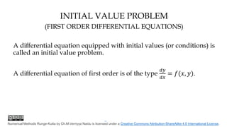
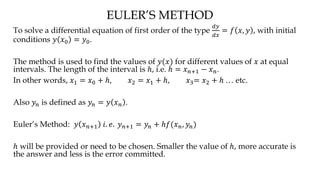
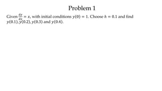
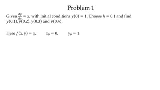
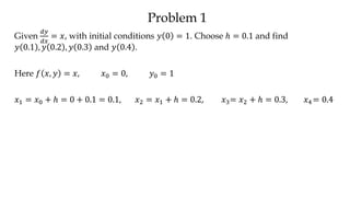
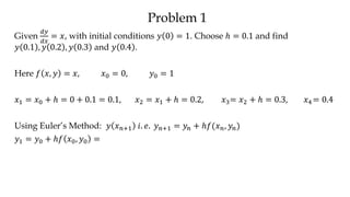
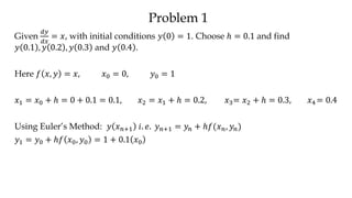
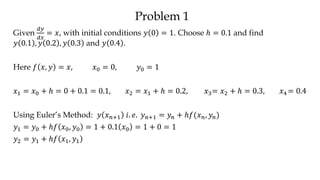
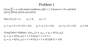
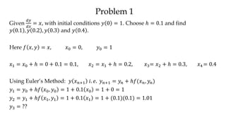
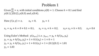
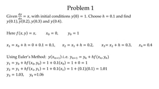
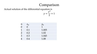
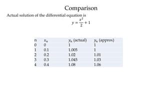
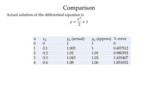
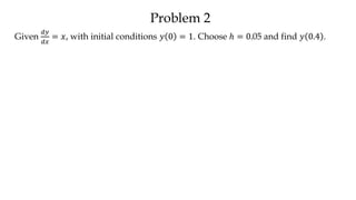
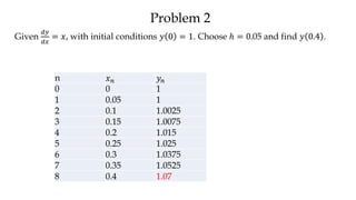
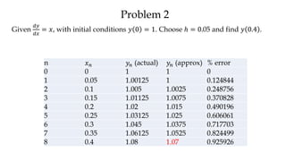
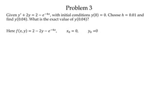
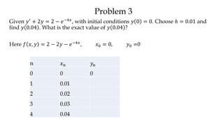
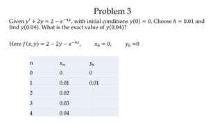
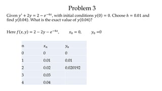
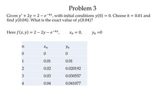
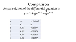
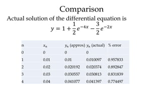
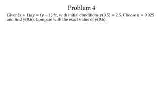
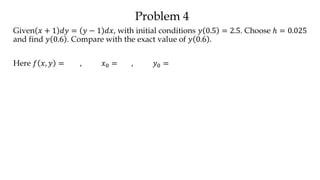
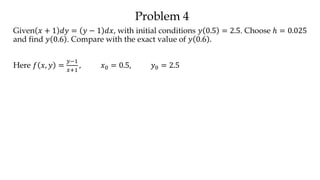
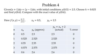
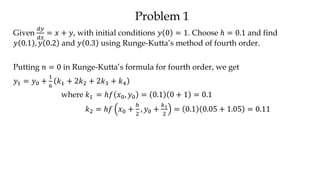
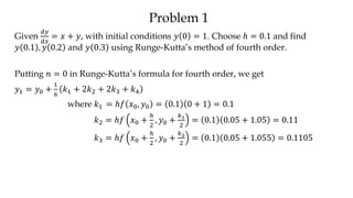
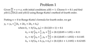
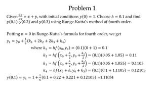
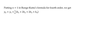
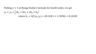
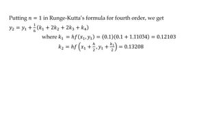
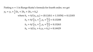
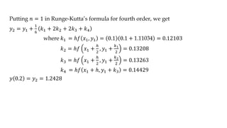
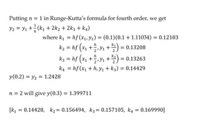
The document discusses initial value problems for first order differential equations and Euler's method for solving such problems numerically. It provides an example problem where Euler's method is used to find successive y-values for the differential equation dy/dx = x with the initial condition y(0) = 1. The y-values found using Euler's method are then compared to the actual solution, showing small errors that decrease as the step size h is reduced.

1. INITIAL VALUE PROBLEM
(FIRST ORDER DIFFERENTIAL EQUATIONS)
A differential equation equipped with initial values (or conditions) is
called an initial value problem.
A differential equation of first order is of the type
𝑑𝑦
𝑑𝑥
= 𝑓(𝑥, 𝑦).

2. INITIAL VALUE PROBLEM
(FIRST ORDER DIFFERENTIAL EQUATIONS)
A differential equation equipped with initial values (or conditions) is
called an initial value problem.
A differential equation of first order is of the type
𝑑𝑦
𝑑𝑥
= 𝑓(𝑥, 𝑦).

3. INITIAL VALUE PROBLEM
(FIRST ORDER DIFFERENTIAL EQUATIONS)
A differential equation equipped with initial values (or conditions) is
called an initial value problem.
A differential equation of first order is of the type
𝑑𝑦
𝑑𝑥
= 𝑓(𝑥, 𝑦).

4. INITIAL VALUE PROBLEM
(FIRST ORDER DIFFERENTIAL EQUATIONS)
A differential equation equipped with initial values (or conditions) is
called an initial value problem.
A differential equation of first order is of the type
𝑑𝑦
𝑑𝑥
= 𝑓(𝑥, 𝑦).
Numerical Methods Runge-Kutta by Ch.M.Verriyya Naidu is licensed under a Creative Commons Attribution-ShareAlike 4.0 International License.

5. EULER’S METHOD
To solve a differential equation of first order of the type
𝑑𝑦
𝑑𝑥
= 𝑓 𝑥, 𝑦 , with initial
conditions 𝑦 𝑥0 = 𝑦0.
The method is used to find the values of 𝑦(𝑥) for different values of 𝑥 at equal
intervals. The length of the interval is ℎ, i.e. ℎ = 𝑥 𝑛+1 − 𝑥 𝑛.
In other words, 𝑥1 = 𝑥0 + ℎ, 𝑥2 = 𝑥1 + ℎ, 𝑥3= 𝑥2 + ℎ … etc.
Also 𝑦𝑛 is defined as 𝑦𝑛 = 𝑦 𝑥 𝑛 .
Euler’s Method: 𝑦 𝑥 𝑛+1 𝑖. 𝑒. 𝑦 𝑛+1 = 𝑦𝑛 + ℎ𝑓(𝑥 𝑛, 𝑦𝑛)
ℎ will be provided or need to be chosen. Smaller the value of ℎ, more accurate is
the answer and less is the error committed.

6. Problem 1
Given
𝑑𝑦
𝑑𝑥
= 𝑥, with initial conditions 𝑦 0 = 1. Choose ℎ = 0.1 and find
𝑦 0.1 , 𝑦 0.2 , 𝑦 0.3 and 𝑦 0.4 .

7. Problem 1
Given
𝑑𝑦
𝑑𝑥
= 𝑥, with initial conditions 𝑦 0 = 1. Choose ℎ = 0.1 and find
𝑦 0.1 , 𝑦 0.2 , 𝑦 0.3 and 𝑦 0.4 .
Here 𝑓 𝑥, 𝑦 = 𝑥, 𝑥0 = 0, 𝑦0 = 1

8. Problem 1
Given
𝑑𝑦
𝑑𝑥
= 𝑥, with initial conditions 𝑦 0 = 1. Choose ℎ = 0.1 and find
𝑦 0.1 , 𝑦 0.2 , 𝑦 0.3 and 𝑦 0.4 .
Here 𝑓 𝑥, 𝑦 = 𝑥, 𝑥0 = 0, 𝑦0 = 1
𝑥1 = 𝑥0 + ℎ = 0 + 0.1 = 0.1, 𝑥2 = 𝑥1 + ℎ = 0.2, 𝑥3= 𝑥2 + ℎ = 0.3, 𝑥4 = 0.4

9. Problem 1
Given
𝑑𝑦
𝑑𝑥
= 𝑥, with initial conditions 𝑦 0 = 1. Choose ℎ = 0.1 and find
𝑦 0.1 , 𝑦 0.2 , 𝑦 0.3 and 𝑦 0.4 .
Here 𝑓 𝑥, 𝑦 = 𝑥, 𝑥0 = 0, 𝑦0 = 1
𝑥1 = 𝑥0 + ℎ = 0 + 0.1 = 0.1, 𝑥2 = 𝑥1 + ℎ = 0.2, 𝑥3= 𝑥2 + ℎ = 0.3, 𝑥4 = 0.4
Using Euler’s Method: 𝑦 𝑥 𝑛+1 𝑖. 𝑒. 𝑦 𝑛+1 = 𝑦𝑛 + ℎ𝑓(𝑥 𝑛, 𝑦𝑛)
𝑦1 = 𝑦0 + ℎ𝑓 𝑥0, 𝑦0 =

10. Problem 1
Given
𝑑𝑦
𝑑𝑥
= 𝑥, with initial conditions 𝑦 0 = 1. Choose ℎ = 0.1 and find
𝑦 0.1 , 𝑦 0.2 , 𝑦 0.3 and 𝑦 0.4 .
Here 𝑓 𝑥, 𝑦 = 𝑥, 𝑥0 = 0, 𝑦0 = 1
𝑥1 = 𝑥0 + ℎ = 0 + 0.1 = 0.1, 𝑥2 = 𝑥1 + ℎ = 0.2, 𝑥3= 𝑥2 + ℎ = 0.3, 𝑥4 = 0.4
Using Euler’s Method: 𝑦 𝑥 𝑛+1 𝑖. 𝑒. 𝑦 𝑛+1 = 𝑦𝑛 + ℎ𝑓(𝑥 𝑛, 𝑦𝑛)
𝑦1 = 𝑦0 + ℎ𝑓 𝑥0, 𝑦0 = 1 + 0.1 𝑥0

11. Problem 1
Given
𝑑𝑦
𝑑𝑥
= 𝑥, with initial conditions 𝑦 0 = 1. Choose ℎ = 0.1 and find
𝑦 0.1 , 𝑦 0.2 , 𝑦 0.3 and 𝑦 0.4 .
Here 𝑓 𝑥, 𝑦 = 𝑥, 𝑥0 = 0, 𝑦0 = 1
𝑥1 = 𝑥0 + ℎ = 0 + 0.1 = 0.1, 𝑥2 = 𝑥1 + ℎ = 0.2, 𝑥3= 𝑥2 + ℎ = 0.3, 𝑥4 = 0.4
Using Euler’s Method: 𝑦 𝑥 𝑛+1 𝑖. 𝑒. 𝑦 𝑛+1 = 𝑦𝑛 + ℎ𝑓(𝑥 𝑛, 𝑦𝑛)
𝑦1 = 𝑦0 + ℎ𝑓 𝑥0, 𝑦0 = 1 + 0.1 𝑥0 = 1 + 0 = 1
𝑦2 = 𝑦1 + ℎ𝑓 𝑥1, 𝑦1

12. Problem 1
Given
𝑑𝑦
𝑑𝑥
= 𝑥, with initial conditions 𝑦 0 = 1. Choose ℎ = 0.1 and find
𝑦 0.1 , 𝑦 0.2 , 𝑦 0.3 and 𝑦 0.4 .
Here 𝑓 𝑥, 𝑦 = 𝑥, 𝑥0 = 0, 𝑦0 = 1
𝑥1 = 𝑥0 + ℎ = 0 + 0.1 = 0.1, 𝑥2 = 𝑥1 + ℎ = 0.2, 𝑥3= 𝑥2 + ℎ = 0.3, 𝑥4 = 0.4
Using Euler’s Method: 𝑦 𝑥 𝑛+1 𝑖. 𝑒. 𝑦 𝑛+1 = 𝑦𝑛 + ℎ𝑓(𝑥 𝑛, 𝑦𝑛)
𝑦1 = 𝑦0 + ℎ𝑓 𝑥0, 𝑦0 = 1 + 0.1 𝑥0 = 1 + 0 = 1
𝑦2 = 𝑦1 + ℎ𝑓 𝑥1, 𝑦1 = 1 + 0.1 𝑥1 = 1 + (0.1)(0.1) = 1.01

13. Problem 1
Given
𝑑𝑦
𝑑𝑥
= 𝑥, with initial conditions 𝑦 0 = 1. Choose ℎ = 0.1 and find
𝑦 0.1 , 𝑦 0.2 , 𝑦 0.3 and 𝑦 0.4 .
Here 𝑓 𝑥, 𝑦 = 𝑥, 𝑥0 = 0, 𝑦0 = 1
𝑥1 = 𝑥0 + ℎ = 0 + 0.1 = 0.1, 𝑥2 = 𝑥1 + ℎ = 0.2, 𝑥3= 𝑥2 + ℎ = 0.3, 𝑥4 = 0.4
Using Euler’s Method: 𝑦 𝑥 𝑛+1 𝑖. 𝑒. 𝑦 𝑛+1 = 𝑦𝑛 + ℎ𝑓(𝑥 𝑛, 𝑦𝑛)
𝑦1 = 𝑦0 + ℎ𝑓 𝑥0, 𝑦0 = 1 + 0.1 𝑥0 = 1 + 0 = 1
𝑦2 = 𝑦1 + ℎ𝑓 𝑥1, 𝑦1 = 1 + 0.1 𝑥1 = 1 + (0.1)(0.1) = 1.01
𝑦3 = ??

14. Problem 1
Given
𝑑𝑦
𝑑𝑥
= 𝑥, with initial conditions 𝑦 0 = 1. Choose ℎ = 0.1 and find
𝑦 0.1 , 𝑦 0.2 , 𝑦 0.3 and 𝑦 0.4 .
Here 𝑓 𝑥, 𝑦 = 𝑥, 𝑥0 = 0, 𝑦0 = 1
𝑥1 = 𝑥0 + ℎ = 0 + 0.1 = 0.1, 𝑥2 = 𝑥1 + ℎ = 0.2, 𝑥3= 𝑥2 + ℎ = 0.3, 𝑥4 = 0.4
Using Euler’s Method: 𝑦 𝑥 𝑛+1 𝑖. 𝑒. 𝑦 𝑛+1 = 𝑦𝑛 + ℎ𝑓(𝑥 𝑛, 𝑦𝑛)
𝑦1 = 𝑦0 + ℎ𝑓 𝑥0, 𝑦0 = 1 + 0.1 𝑥0 = 1 + 0 = 1
𝑦2 = 𝑦1 + ℎ𝑓 𝑥1, 𝑦1 = 1 + 0.1 𝑥1 = 1 + (0.1)(0.1) = 1.01
𝑦3 = 1.03

15. Problem 1
Given
𝑑𝑦
𝑑𝑥
= 𝑥, with initial conditions 𝑦 0 = 1. Choose ℎ = 0.1 and find
𝑦 0.1 , 𝑦 0.2 , 𝑦 0.3 and 𝑦 0.4 .
Here 𝑓 𝑥, 𝑦 = 𝑥, 𝑥0 = 0, 𝑦0 = 1
𝑥1 = 𝑥0 + ℎ = 0 + 0.1 = 0.1, 𝑥2 = 𝑥1 + ℎ = 0.2, 𝑥3= 𝑥2 + ℎ = 0.3, 𝑥4 = 0.4
Using Euler’s Method: 𝑦 𝑥 𝑛+1 𝑖. 𝑒. 𝑦 𝑛+1 = 𝑦𝑛 + ℎ𝑓(𝑥 𝑛, 𝑦𝑛)
𝑦1 = 𝑦0 + ℎ𝑓 𝑥0, 𝑦0 = 1 + 0.1 𝑥0 = 1 + 0 = 1
𝑦2 = 𝑦1 + ℎ𝑓 𝑥1, 𝑦1 = 1 + 0.1 𝑥1 = 1 + (0.1)(0.1) = 1.01
𝑦3 = 1.03, 𝑦4 =1.06

16. Comparison
Actual solution of the differential equation is
𝑦 =
𝑥2
2
+ 1
n 𝑥 𝑛 𝑦𝑛
0 0 1
1 0.1 1.005
2 0.2 1.02
3 0.3 1.045
4 0.4 1.08

17. Comparison
Actual solution of the differential equation is
𝑦 =
𝑥2
2
+ 1
n 𝑥 𝑛 𝑦𝑛 (actual) 𝑦𝑛 (approx)
0 0 1 1
1 0.1 1.005 1
2 0.2 1.02 1.01
3 0.3 1.045 1.03
4 0.4 1.08 1.06

18. Comparison
Actual solution of the differential equation is
𝑦 =
𝑥2
2
+ 1
n 𝑥 𝑛 𝑦𝑛 (actual) 𝑦𝑛 (approx) % error
0 0 1 1 0
1 0.1 1.005 1 0.497512
2 0.2 1.02 1.01 0.980392
3 0.3 1.045 1.03 1.435407
4 0.4 1.08 1.06 1.851852

19. Problem 2
Given
𝑑𝑦
𝑑𝑥
= 𝑥, with initial conditions 𝑦 0 = 1. Choose ℎ = 0.05 and find 𝑦 0.4 .

20. Problem 2
Given
𝑑𝑦
𝑑𝑥
= 𝑥, with initial conditions 𝑦 0 = 1. Choose ℎ = 0.05 and find 𝑦 0.4 .
n 𝑥 𝑛 𝑦𝑛
0 0 1
1 0.05 1
2 0.1 1.0025
3 0.15 1.0075
4 0.2 1.015
5 0.25 1.025
6 0.3 1.0375
7 0.35 1.0525
8 0.4 1.07

21. Problem 2
Given
𝑑𝑦
𝑑𝑥
= 𝑥, with initial conditions 𝑦 0 = 1. Choose ℎ = 0.05 and find 𝑦 0.4 .
n 𝑥 𝑛 𝑦𝑛 (actual) 𝑦𝑛 (approx) % error
0 0 1 1 0
1 0.05 1.00125 1 0.124844
2 0.1 1.005 1.0025 0.248756
3 0.15 1.01125 1.0075 0.370828
4 0.2 1.02 1.015 0.490196
5 0.25 1.03125 1.025 0.606061
6 0.3 1.045 1.0375 0.717703
7 0.35 1.06125 1.0525 0.824499
8 0.4 1.08 1.07 0.925926

22. Problem 3
Given 𝑦′ + 2𝑦 = 2 − 𝑒−4𝑥, with initial conditions 𝑦 0 = 0. Choose ℎ = 0.01 and
find 𝑦 0.04 . What is the exact value of 𝑦 0.04 ?

23. Problem 3
Given 𝑦′ + 2𝑦 = 2 − 𝑒−4𝑥, with initial conditions 𝑦 0 = 0. Choose ℎ = 0.01 and
find 𝑦 0.04 . What is the exact value of 𝑦 0.04 ?
Here 𝑓 𝑥, 𝑦 = 2 − 2𝑦 − 𝑒−4𝑥, 𝑥0 = 0, 𝑦0 =0

24. Problem 3
Given 𝑦′ + 2𝑦 = 2 − 𝑒−4𝑥, with initial conditions 𝑦 0 = 0. Choose ℎ = 0.01 and
find 𝑦 0.04 . What is the exact value of 𝑦 0.04 ?
Here 𝑓 𝑥, 𝑦 = 2 − 2𝑦 − 𝑒−4𝑥, 𝑥0 = 0, 𝑦0 =0
n 𝑥 𝑛 𝑦𝑛
0 0 0
1 0.01
2 0.02
3 0.03
4 0.04

25. Problem 3
Given 𝑦′ + 2𝑦 = 2 − 𝑒−4𝑥, with initial conditions 𝑦 0 = 0. Choose ℎ = 0.01 and
find 𝑦 0.04 . What is the exact value of 𝑦 0.04 ?
Here 𝑓 𝑥, 𝑦 = 2 − 2𝑦 − 𝑒−4𝑥, 𝑥0 = 0, 𝑦0 =0
n 𝑥 𝑛 𝑦𝑛
0 0 0
1 0.01 0.01
2 0.02
3 0.03
4 0.04

26. Problem 3
Given 𝑦′ + 2𝑦 = 2 − 𝑒−4𝑥, with initial conditions 𝑦 0 = 0. Choose ℎ = 0.01 and
find 𝑦 0.04 . What is the exact value of 𝑦 0.04 ?
Here 𝑓 𝑥, 𝑦 = 2 − 2𝑦 − 𝑒−4𝑥, 𝑥0 = 0, 𝑦0 =0
n 𝑥 𝑛 𝑦𝑛
0 0 0
1 0.01 0.01
2 0.02 0.020192
3 0.03
4 0.04

27. Problem 3
Given 𝑦′ + 2𝑦 = 2 − 𝑒−4𝑥, with initial conditions 𝑦 0 = 0. Choose ℎ = 0.01 and
find 𝑦 0.04 . What is the exact value of 𝑦 0.04 ?
Here 𝑓 𝑥, 𝑦 = 2 − 2𝑦 − 𝑒−4𝑥, 𝑥0 = 0, 𝑦0 =0
n 𝑥 𝑛 𝑦𝑛
0 0 0
1 0.01 0.01
2 0.02 0.020192
3 0.03 0.030557
4 0.04 0.041077

28. Comparison
Actual solution of the differential equation is
𝑦 = 1 +
1
2
𝑒−4𝑥
−
3
2
𝑒−2𝑥
n 𝑥 𝑛 𝑦𝑛 (actual)
0 0 0
1 0.01 0.010097
2 0.02 0.020374
3 0.03 0.030813
4 0.04 0.041397

29. Comparison
Actual solution of the differential equation is
𝑦 = 1 +
1
2
𝑒−4𝑥
−
3
2
𝑒−2𝑥
n 𝑥 𝑛 𝑦𝑛 (approx) 𝑦𝑛 (actual) % error
0 0 0 0
1 0.01 0.01 0.010097 0.957833
2 0.02 0.020192 0.020374 0.892847
3 0.03 0.030557 0.030813 0.831839
4 0.04 0.041077 0.041397 0.774497

30. Problem 4
Given 𝑥 + 1 𝑑𝑦 = 𝑦 − 1 𝑑𝑥, with initial conditions 𝑦 0.5 = 2.5. Choose ℎ = 0.025
and find 𝑦 0.6 . Compare with the exact value of 𝑦 0.6 .

31. Problem 4
Given 𝑥 + 1 𝑑𝑦 = 𝑦 − 1 𝑑𝑥, with initial conditions 𝑦 0.5 = 2.5. Choose ℎ = 0.025
and find 𝑦 0.6 . Compare with the exact value of 𝑦 0.6 .
Here 𝑓 𝑥, 𝑦 = , 𝑥0 = , 𝑦0 =

32. Problem 4
Given 𝑥 + 1 𝑑𝑦 = 𝑦 − 1 𝑑𝑥, with initial conditions 𝑦 0.5 = 2.5. Choose ℎ = 0.025
and find 𝑦 0.6 . Compare with the exact value of 𝑦 0.6 .
Here 𝑓 𝑥, 𝑦 =
𝑦−1
𝑥+1
, 𝑥0 = 0.5, 𝑦0 = 2.5

33. Problem 4
Given 𝑥 + 1 𝑑𝑦 = 𝑦 − 1 𝑑𝑥, with initial conditions 𝑦 0.5 = 2.5. Choose ℎ = 0.025
and find 𝑦 0.6 . Compare with the exact value of 𝑦 0.6 .
Here 𝑓 𝑥, 𝑦 =
𝑦−1
𝑥+1
, 𝑥0 = 0.5, 𝑦0 = 2.5
n 𝑥 𝑛 𝑦𝑛 (approx)
𝑦𝑛 = 𝑥 𝑛 + 2
(actual) % error
0 0.5 2.5 2.5 0
1 0.525 2.525 2.525 0
2 0.55 2.55 2.55 0
3 0.575 2.575 2.575 0
4 0.6 2.6 2.6 0

34. RUNGE-KUTTA’S METHOD
1. Second order
𝑦 𝑛+1 = 𝑦𝑛 +
1
2
𝑘1 + 𝑘2
where 𝑘1 = ℎ𝑓 𝑥 𝑛, 𝑦𝑛
𝑘2 = ℎ𝑓 𝑥 𝑛 + ℎ, 𝑦𝑛 + 𝑘1
2. Fourth order
𝑦 𝑛+1 = 𝑦𝑛 +
1
6
𝑘1 + 2𝑘2 + 2𝑘3 + 𝑘4
where 𝑘1 = ℎ𝑓 𝑥 𝑛, 𝑦𝑛
𝑘2 = ℎ𝑓 𝑥 𝑛 +
ℎ
2
, 𝑦𝑛 +
𝑘1
2
𝑘3 = ℎ𝑓 𝑥 𝑛 +
ℎ
2
, 𝑦𝑛 +
𝑘2
2
𝑘4 = ℎ𝑓 𝑥 𝑛 + ℎ, 𝑦𝑛 + 𝑘3

35. Problem 1
Given
𝑑𝑦
𝑑𝑥
= 𝑥 + 𝑦, with initial conditions 𝑦 0 = 1. Choose ℎ = 0.1 and find
𝑦 0.1 , 𝑦 0.2 and 𝑦 0.3 using Runge-Kutta’s method of fourth order.

36. Problem 1
Given
𝑑𝑦
𝑑𝑥
= 𝑥 + 𝑦, with initial conditions 𝑦 0 = 1. Choose ℎ = 0.1 and find
𝑦 0.1 , 𝑦 0.2 and 𝑦 0.3 using Runge-Kutta’s method of fourth order.
Putting 𝑛 = 0 in Runge-Kutta’s formula for fourth order, we get

37. Problem 1
Given
𝑑𝑦
𝑑𝑥
= 𝑥 + 𝑦, with initial conditions 𝑦 0 = 1. Choose ℎ = 0.1 and find
𝑦 0.1 , 𝑦 0.2 and 𝑦 0.3 using Runge-Kutta’s method of fourth order.
Putting 𝑛 = 0 in Runge-Kutta’s formula for fourth order, we get
𝑦1 = 𝑦0 +
1
6
𝑘1 + 2𝑘2 + 2𝑘3 + 𝑘4

38. Problem 1
Given
𝑑𝑦
𝑑𝑥
= 𝑥 + 𝑦, with initial conditions 𝑦 0 = 1. Choose ℎ = 0.1 and find
𝑦 0.1 , 𝑦 0.2 and 𝑦 0.3 using Runge-Kutta’s method of fourth order.
Putting 𝑛 = 0 in Runge-Kutta’s formula for fourth order, we get
𝑦1 = 𝑦0 +
1
6
𝑘1 + 2𝑘2 + 2𝑘3 + 𝑘4
where 𝑘1 = ℎ𝑓 𝑥0, 𝑦0 = 0.1 0 + 1 = 0.1

39. Problem 1
Given
𝑑𝑦
𝑑𝑥
= 𝑥 + 𝑦, with initial conditions 𝑦 0 = 1. Choose ℎ = 0.1 and find
𝑦 0.1 , 𝑦 0.2 and 𝑦 0.3 using Runge-Kutta’s method of fourth order.
Putting 𝑛 = 0 in Runge-Kutta’s formula for fourth order, we get
𝑦1 = 𝑦0 +
1
6
𝑘1 + 2𝑘2 + 2𝑘3 + 𝑘4
where 𝑘1 = ℎ𝑓 𝑥0, 𝑦0 = 0.1 0 + 1 = 0.1
𝑘2 = ℎ𝑓 𝑥0 +
ℎ
2
, 𝑦0 +
𝑘1
2
= 0.1 0.05 + 1.05 = 0.11

40. Problem 1
Given
𝑑𝑦
𝑑𝑥
= 𝑥 + 𝑦, with initial conditions 𝑦 0 = 1. Choose ℎ = 0.1 and find
𝑦 0.1 , 𝑦 0.2 and 𝑦 0.3 using Runge-Kutta’s method of fourth order.
Putting 𝑛 = 0 in Runge-Kutta’s formula for fourth order, we get
𝑦1 = 𝑦0 +
1
6
𝑘1 + 2𝑘2 + 2𝑘3 + 𝑘4
where 𝑘1 = ℎ𝑓 𝑥0, 𝑦0 = 0.1 0 + 1 = 0.1
𝑘2 = ℎ𝑓 𝑥0 +
ℎ
2
, 𝑦0 +
𝑘1
2
= 0.1 0.05 + 1.05 = 0.11
𝑘3 = ℎ𝑓 𝑥0 +
ℎ
2
, 𝑦0 +
𝑘2
2
= 0.1 0.05 + 1.055 = 0.1105

41. Problem 1
Given
𝑑𝑦
𝑑𝑥
= 𝑥 + 𝑦, with initial conditions 𝑦 0 = 1. Choose ℎ = 0.1 and find
𝑦 0.1 , 𝑦 0.2 and 𝑦 0.3 using Runge-Kutta’s method of fourth order.
Putting 𝑛 = 0 in Runge-Kutta’s formula for fourth order, we get
𝑦1 = 𝑦0 +
1
6
𝑘1 + 2𝑘2 + 2𝑘3 + 𝑘4
where 𝑘1 = ℎ𝑓 𝑥0, 𝑦0 = 0.1 0 + 1 = 0.1
𝑘2 = ℎ𝑓 𝑥0 +
ℎ
2
, 𝑦0 +
𝑘1
2
= 0.1 0.05 + 1.05 = 0.11
𝑘3 = ℎ𝑓 𝑥0 +
ℎ
2
, 𝑦0 +
𝑘2
2
= 0.1 0.05 + 1.055 = 0.1105
𝑘4 = ℎ𝑓 𝑥0 + ℎ, 𝑦0 + 𝑘3 = 0.1 0.1 + 1.1105 = 0.12105

42. Problem 1
Given
𝑑𝑦
𝑑𝑥
= 𝑥 + 𝑦, with initial conditions 𝑦 0 = 1. Choose ℎ = 0.1 and find
𝑦 0.1 , 𝑦 0.2 and 𝑦 0.3 using Runge-Kutta’s method of fourth order.
Putting 𝑛 = 0 in Runge-Kutta’s formula for fourth order, we get
𝑦1 = 𝑦0 +
1
6
𝑘1 + 2𝑘2 + 2𝑘3 + 𝑘4
where 𝑘1 = ℎ𝑓 𝑥0, 𝑦0 = 0.1 0 + 1 = 0.1
𝑘2 = ℎ𝑓 𝑥0 +
ℎ
2
, 𝑦0 +
𝑘1
2
= 0.1 0.05 + 1.05 = 0.11
𝑘3 = ℎ𝑓 𝑥0 +
ℎ
2
, 𝑦0 +
𝑘2
2
= 0.1 0.05 + 1.055 = 0.1105
𝑘4 = ℎ𝑓 𝑥0 + ℎ, 𝑦0 + 𝑘3 = 0.1 0.1 + 1.1105 = 0.12105
𝑦 0.1 = 𝑦1 = 1 +
1
6
0.1 + 0.22 + 0.221 + 0.12105 =1.11034

43. Putting 𝑛 = 1 in Runge-Kutta’s formula for fourth order, we get
𝑦2 = 𝑦1 +
1
6
𝑘1 + 2𝑘2 + 2𝑘3 + 𝑘4

44. Putting 𝑛 = 1 in Runge-Kutta’s formula for fourth order, we get
𝑦2 = 𝑦1 +
1
6
𝑘1 + 2𝑘2 + 2𝑘3 + 𝑘4
where 𝑘1 = ℎ𝑓 𝑥1, 𝑦1 = 0.1 0.1 + 1.11034 = 0.12103

45. Putting 𝑛 = 1 in Runge-Kutta’s formula for fourth order, we get
𝑦2 = 𝑦1 +
1
6
𝑘1 + 2𝑘2 + 2𝑘3 + 𝑘4
where 𝑘1 = ℎ𝑓 𝑥1, 𝑦1 = 0.1 0.1 + 1.11034 = 0.12103
𝑘2 = ℎ𝑓 𝑥1 +
ℎ
2
, 𝑦1 +
𝑘1
2
= 0.13208

46. Putting 𝑛 = 1 in Runge-Kutta’s formula for fourth order, we get
𝑦2 = 𝑦1 +
1
6
𝑘1 + 2𝑘2 + 2𝑘3 + 𝑘4
where 𝑘1 = ℎ𝑓 𝑥1, 𝑦1 = 0.1 0.1 + 1.11034 = 0.12103
𝑘2 = ℎ𝑓 𝑥1 +
ℎ
2
, 𝑦1 +
𝑘1
2
= 0.13208
𝑘3 = ℎ𝑓 𝑥1 +
ℎ
2
, 𝑦1 +
𝑘2
2
= 0.13263
𝑘4 = ℎ𝑓 𝑥1 + ℎ, 𝑦1 + 𝑘3 = 0.14429

47. Putting 𝑛 = 1 in Runge-Kutta’s formula for fourth order, we get
𝑦2 = 𝑦1 +
1
6
𝑘1 + 2𝑘2 + 2𝑘3 + 𝑘4
where 𝑘1 = ℎ𝑓 𝑥1, 𝑦1 = 0.1 0.1 + 1.11034 = 0.12103
𝑘2 = ℎ𝑓 𝑥1 +
ℎ
2
, 𝑦1 +
𝑘1
2
= 0.13208
𝑘3 = ℎ𝑓 𝑥1 +
ℎ
2
, 𝑦1 +
𝑘2
2
= 0.13263
𝑘4 = ℎ𝑓 𝑥1 + ℎ, 𝑦1 + 𝑘3 = 0.14429
𝑦 0.2 = 𝑦2 = 1.2428

48. Putting 𝑛 = 1 in Runge-Kutta’s formula for fourth order, we get
𝑦2 = 𝑦1 +
1
6
𝑘1 + 2𝑘2 + 2𝑘3 + 𝑘4
where 𝑘1 = ℎ𝑓 𝑥1, 𝑦1 = 0.1 0.1 + 1.11034 = 0.12103
𝑘2 = ℎ𝑓 𝑥1 +
ℎ
2
, 𝑦1 +
𝑘1
2
= 0.13208
𝑘3 = ℎ𝑓 𝑥1 +
ℎ
2
, 𝑦1 +
𝑘2
2
= 0.13263
𝑘4 = ℎ𝑓 𝑥1 + ℎ, 𝑦1 + 𝑘3 = 0.14429
𝑦 0.2 = 𝑦2 = 1.2428
𝑛 = 2 will give 𝑦 0.3 = 1.399711
𝑘1 = 0.14428, 𝑘2 = 0.156494, 𝑘3 = 0.157105, 𝑘4 = 0.169990