Downloaded 123 times
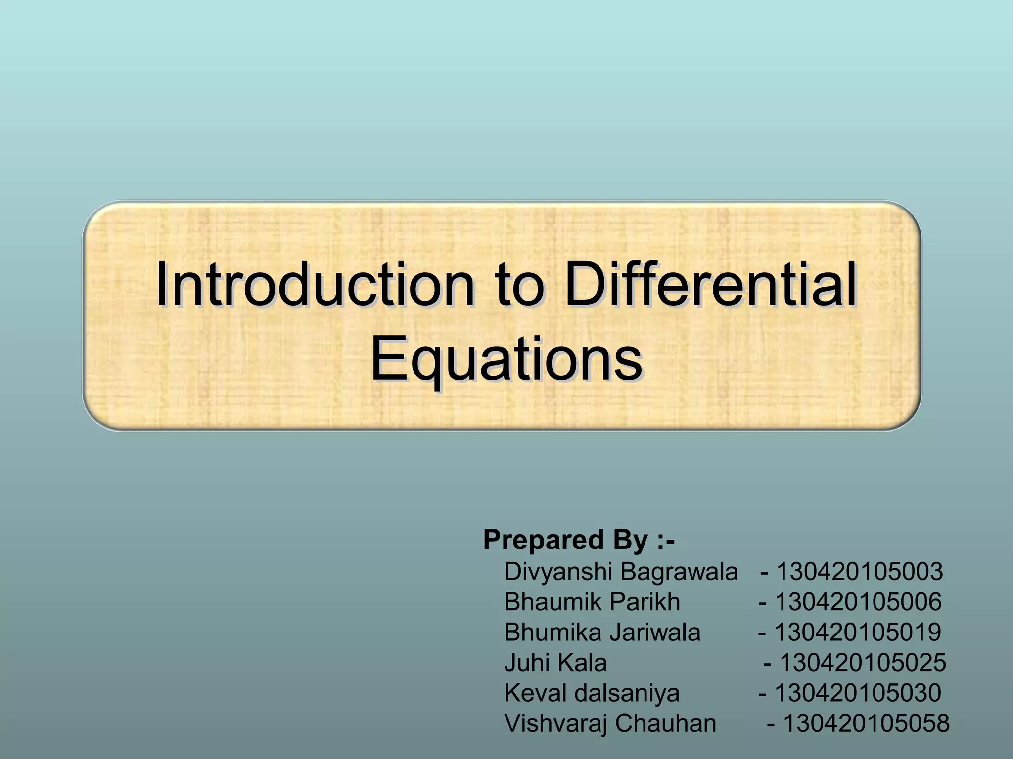
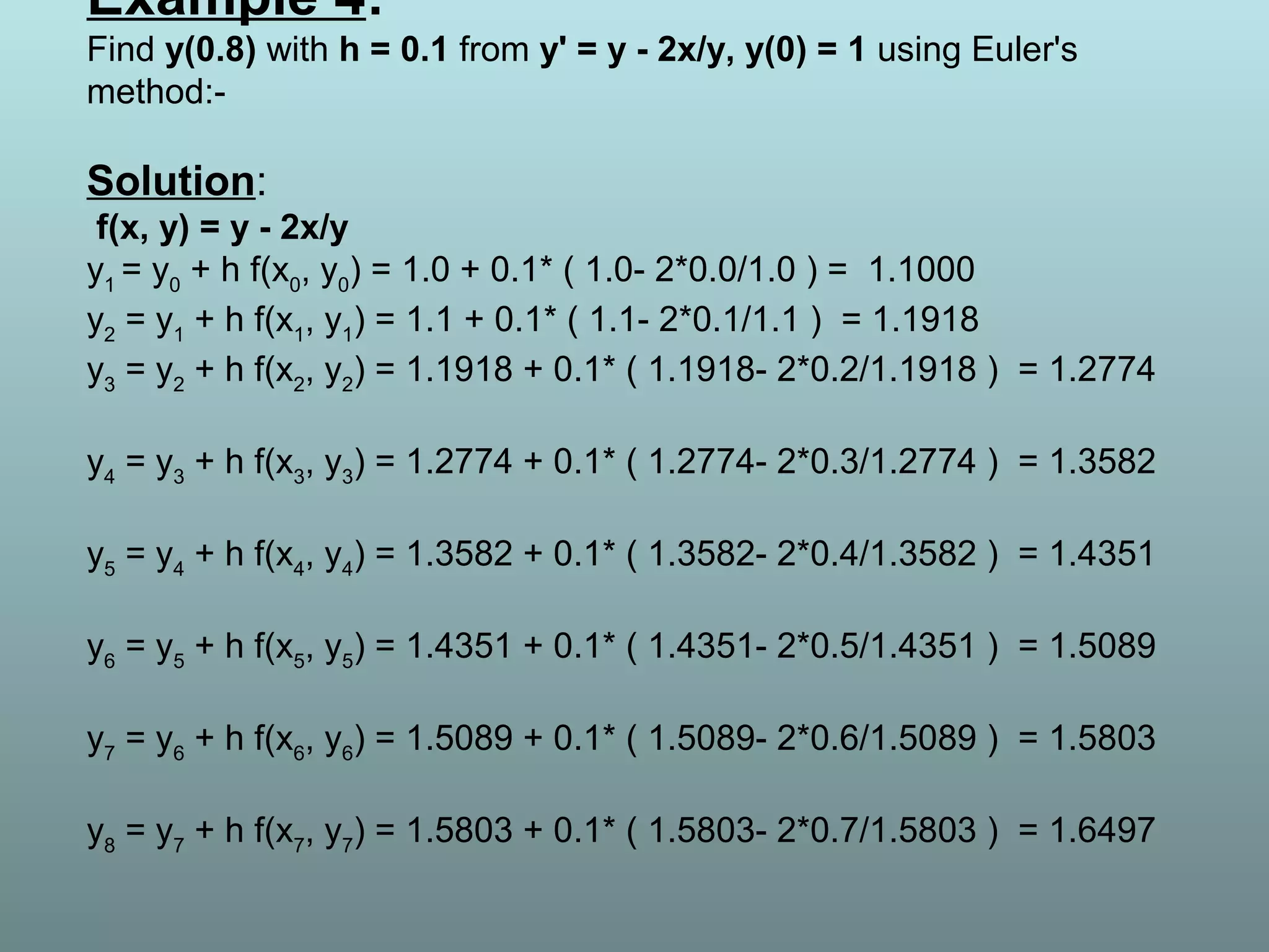
![Example 5:
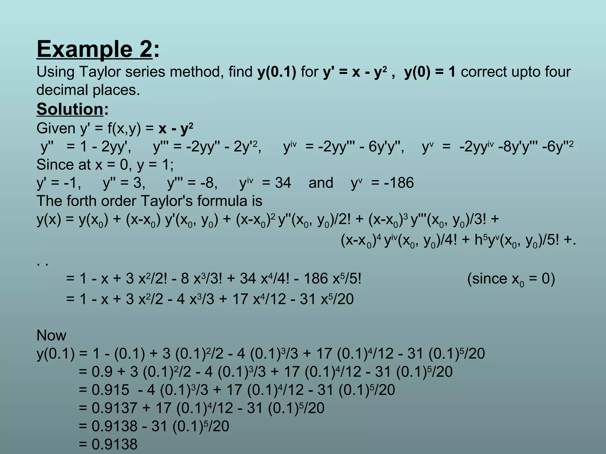
Find y(1.0) accurate upto four decimal places using Modified Euler's
method by solving the IVP y' = -2xy2
, y(0) = 1 with step lengh 0.2.
Solution:
f(x, y) = -2xy2
y' = -2*x*y*y, y[0.0] = 1.0 with h = 0.2
Given
y[0.0] = 1.0
Euler Solution: y(1) = y(0) + h*(-2*x*y*y)(1)
y[0.20] = 1.0
Modified Euler iterations:y(1) = y(0) + .5*h*((-2*x*y*y)(0) + (-2*x*y*y)(1)
y[0.20] = 1.0 y[0.20] = 0.9599999988079071 y[0.20] =
0.9631359989929199
y[0.20] = 0.9628947607919341 y[0.20] = 0.9629133460803093
Euler Solution: y(2) = y(1) + h*(-2*x*y*y)(2)
y[0.40] = 0.8887359638083165
Modified Euler iterations:y(2) = y(1) + .5*h*((-2*x*y*y)(1) + (-2*x*y*y)(2)
y[0.40] = 0.8887359638083165 y[0.40] = 0.8626358081578545
y[0.40] = 0.8662926943348495 y[0.40] = 0.8657868947404332
y[0.40] = 0.865856981554814](https://image.slidesharecdn.com/cem-150430012857-conversion-gate02/75/Introduction-to-Differential-Equations-20-2048.jpg)
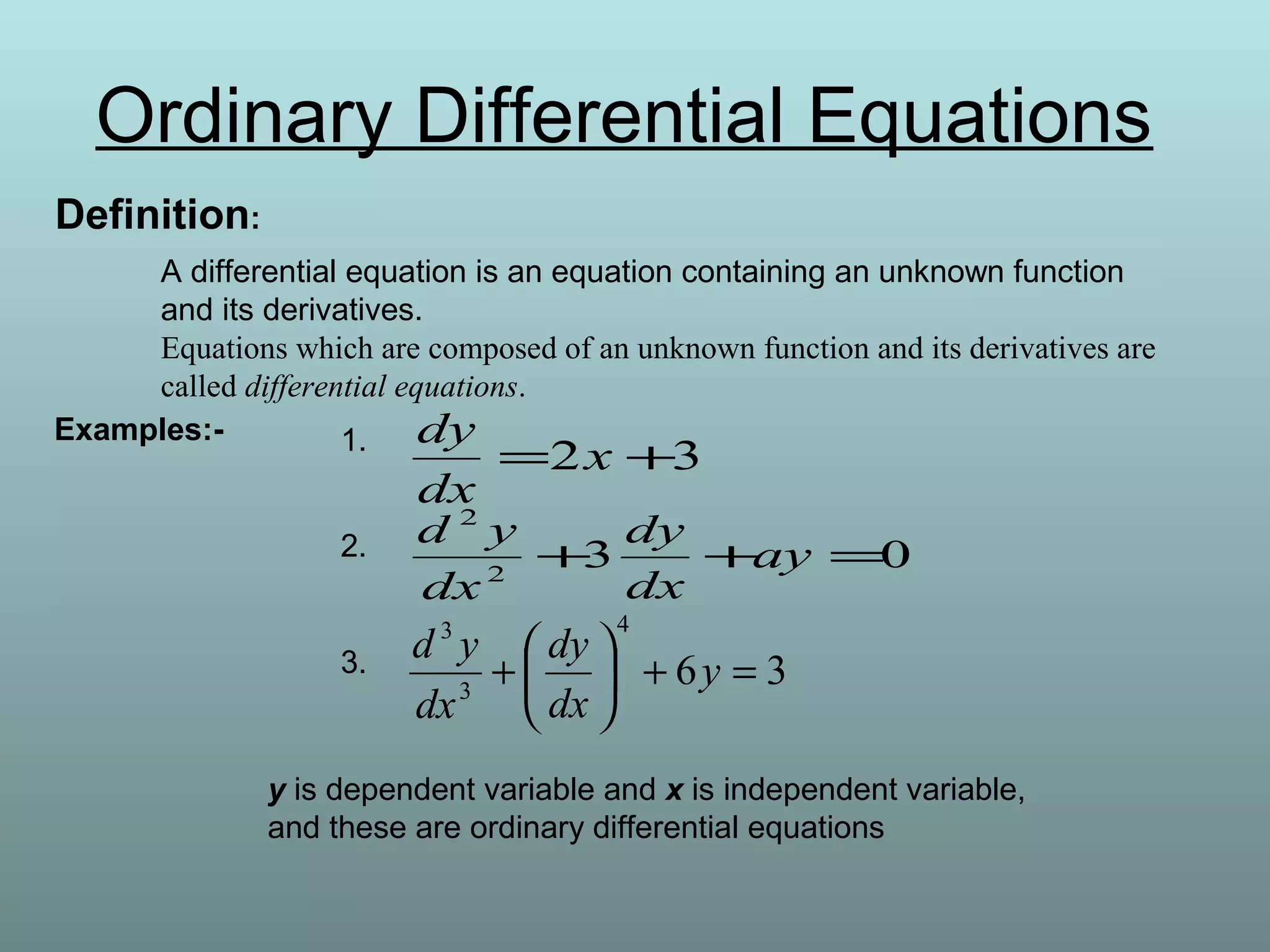
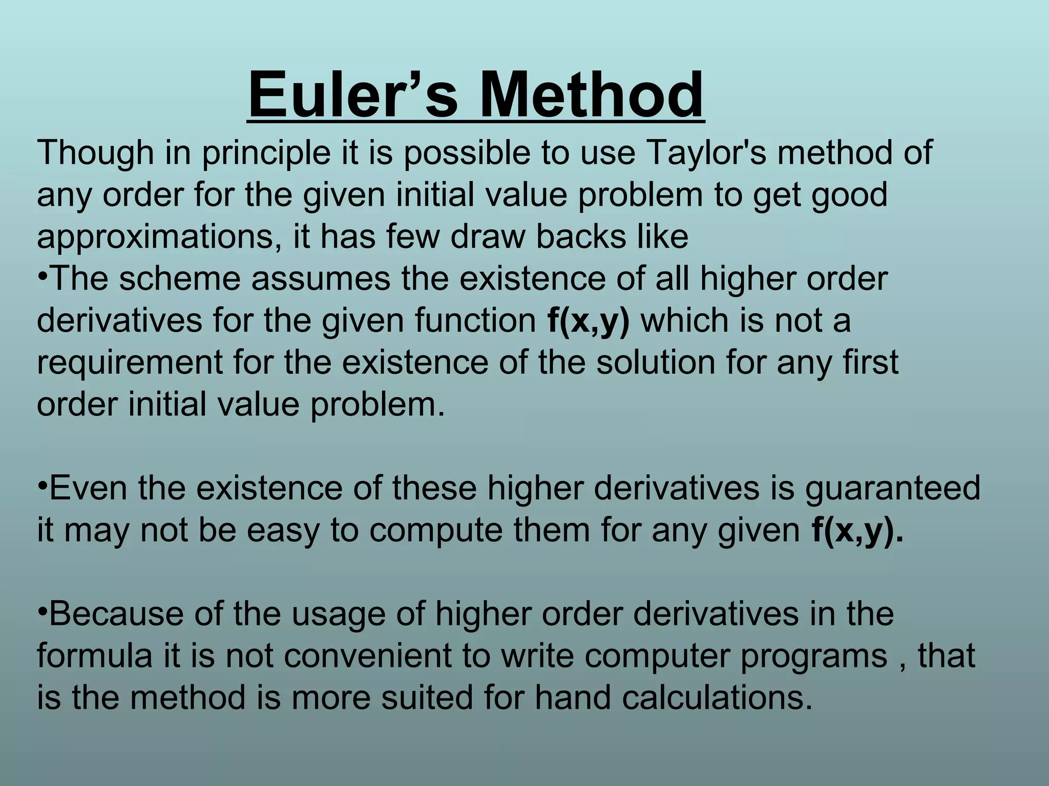
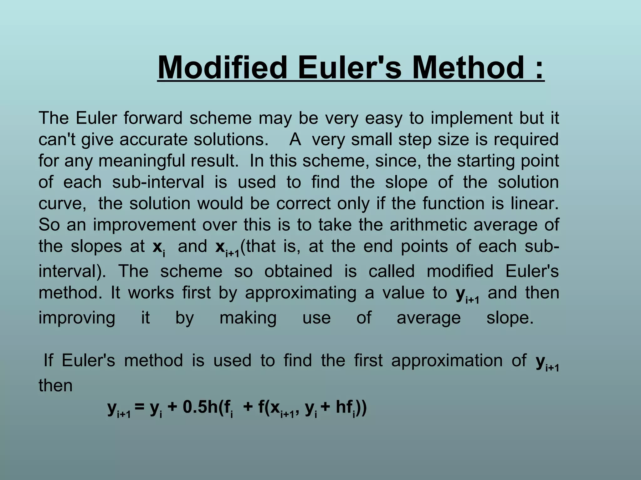
![Euler Solution: y(3) = y(2) + h*(-2*x*y*y)(3)
y[0.60] = 0.7458966289094106
Modified Euler iterations:y(3) = y(2) + .5*h*((-2*x*y*y)(2) + (-2*x*y*y)(3)
y[0.60] = 0.7458966289094106 y[0.60] = 0.7391085349039348
y[0.60] = 0.7403181774980547 y[0.60] = 0.7401034281837107
y[0.60] = 0.7401415785278189
Euler Solution: y(4) = y(3) + h*(-2*x*y*y)(4)
y[0.80] = 0.6086629119889084
Modified Euler iterations:y(4) = y(3) + .5*h*((-2*x*y*y)(3) + (-2*x*y*y)(4)
y[0.80] = 0.6086629119889084 y[0.80] = 0.6151235687114084
y[0.80] = 0.6138585343771569 y[0.80] = 0.6141072871136244
y[0.80] = 0.6140584135348263
Euler Solution: y(5) = y(4) + h*(-2*x*y*y)(5)
y[1.00] = 0.49340256427369866
Modified Euler iterations:y(5) = y(4) + .5*h*((-2*x*y*y)(4) + (-2*x*y*y)(5)
y[1.00] = 0.49340256427369866 y[1.00] = 0.5050460713552334
y[1.00] = 0.5027209825340415 y[1.00] = 0.5031896121302805
y[1.00] = 0.5030953322323046 y[1.00] = 0.503114306721248](https://image.slidesharecdn.com/cem-150430012857-conversion-gate02/75/Introduction-to-Differential-Equations-21-2048.jpg)
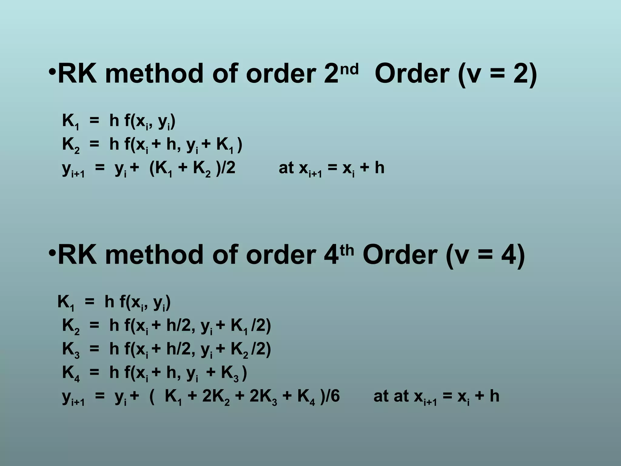
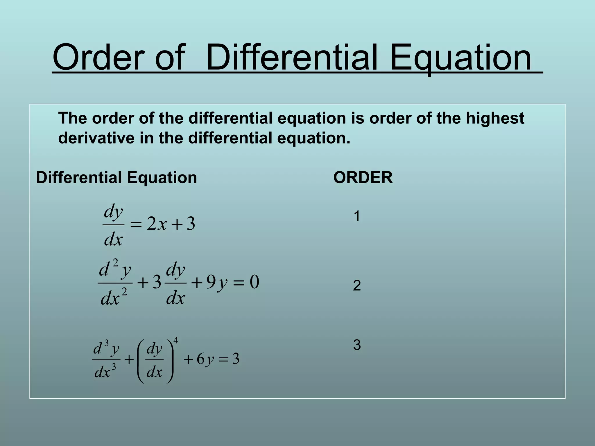
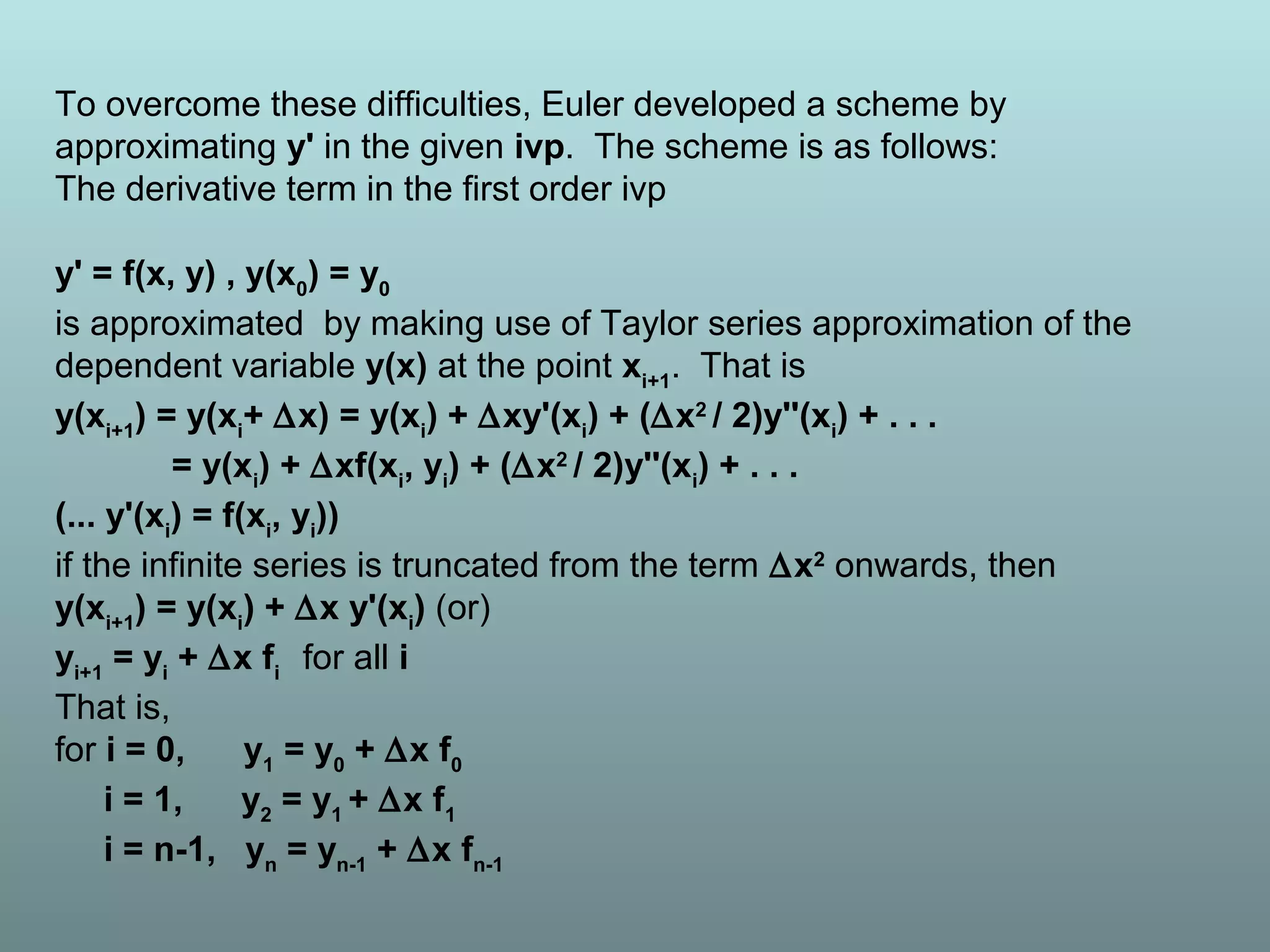
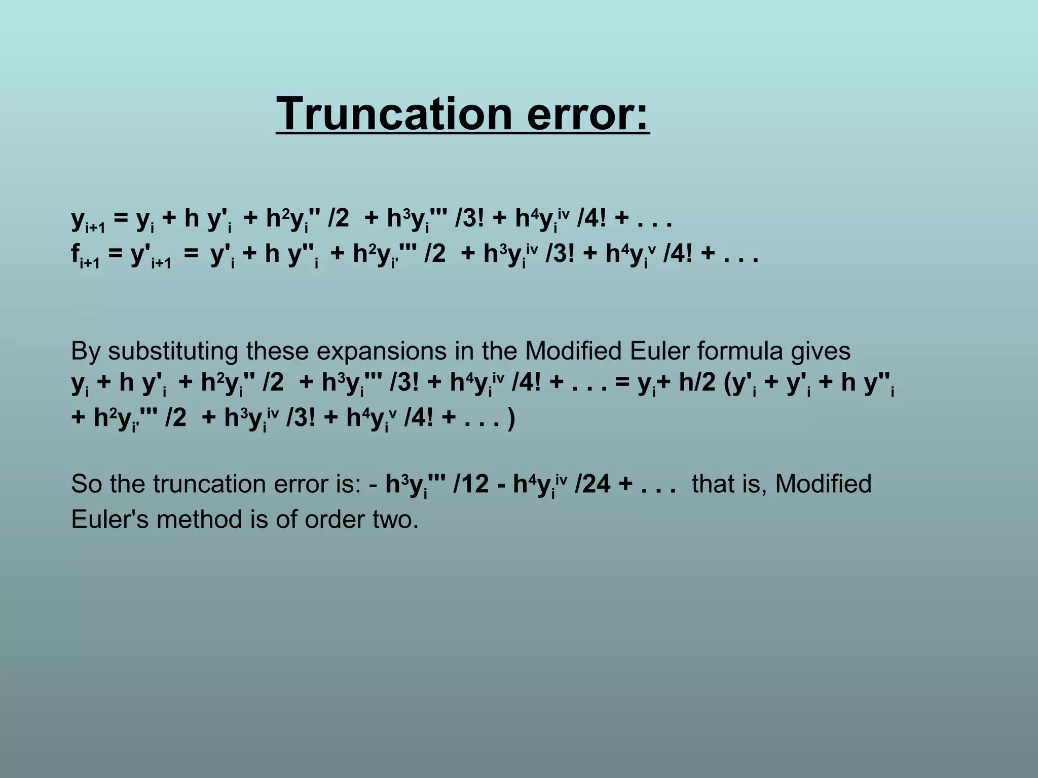
![Example 6:
Using RK method of order four find y at x = 1.1 and 1.2 by solving y' = x2
+
y2
, y(1) = 2.3
Solution: Using RK method of order 4
Given y' = x*x+y*y,
y[1.00] = 2.3
with step-length = 0.1
K1 = 0.628999987438321
K2 = 0.7938110087671021
K3 = 0.83757991687511
K4 = 1.1054407603556848
y[1.10] = 3.1328703854960227
K1 = 1.102487701987972
K2 = 1.4895197934605002
K3 = 1.6358516854539997
K4 = 2.4180710557439085
y[1.20] = 4.761420671422837](https://image.slidesharecdn.com/cem-150430012857-conversion-gate02/75/Introduction-to-Differential-Equations-24-2048.jpg)


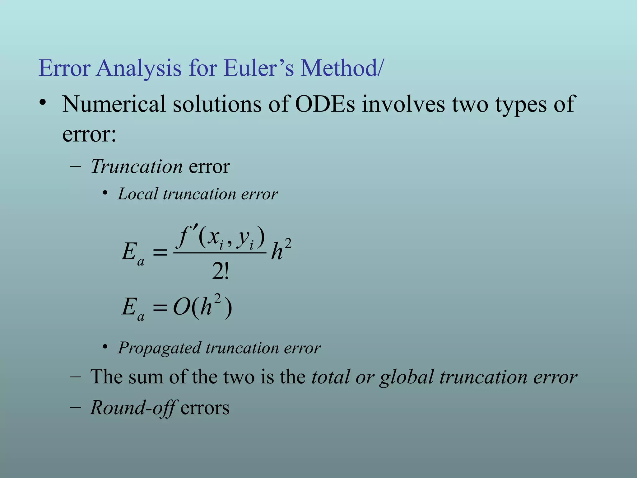
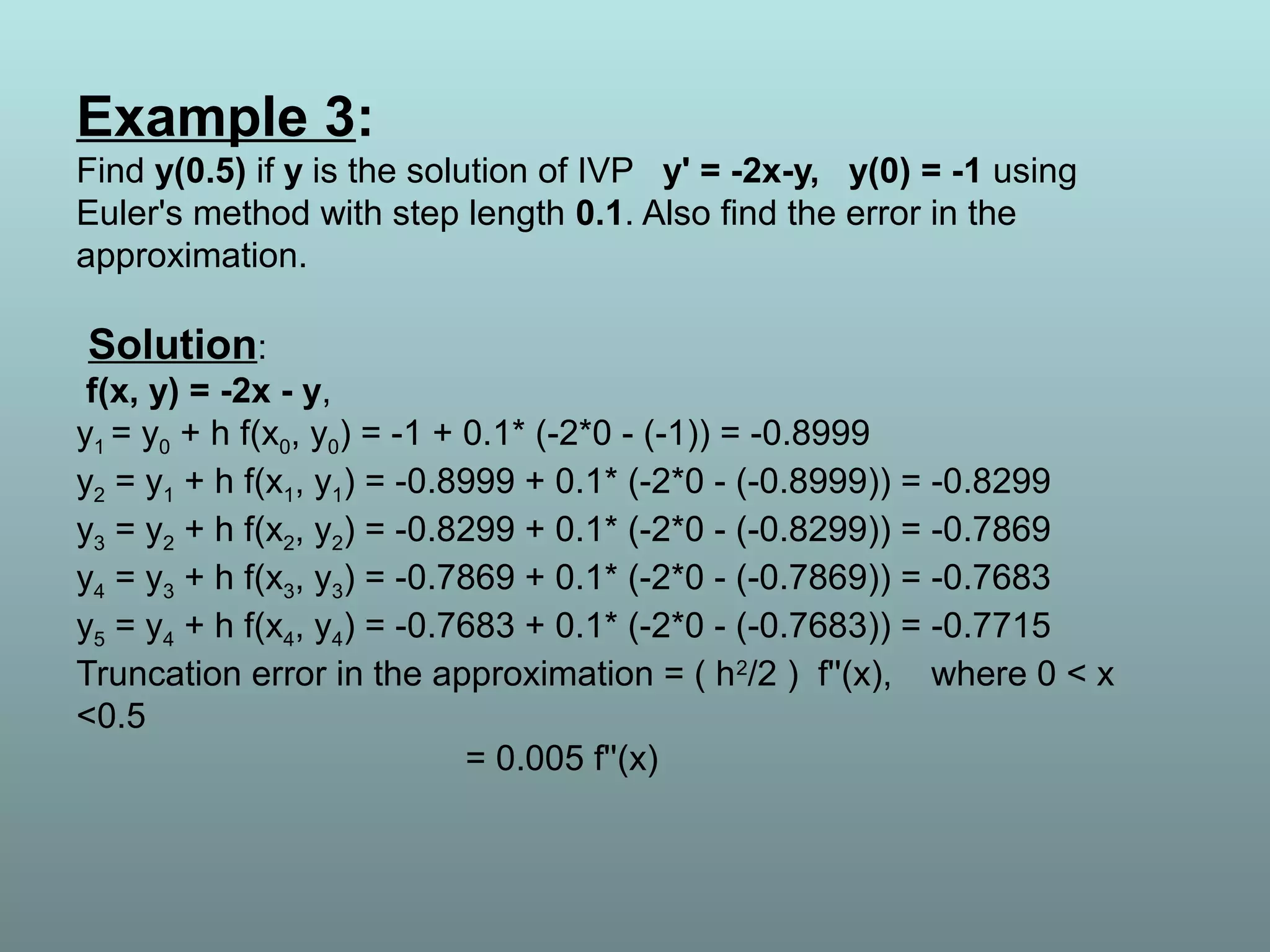
This document provides an introduction to differential equations. It defines a differential equation as an equation containing an unknown function and its derivatives. Ordinary differential equations are presented, along with definitions of the order and degree of a differential equation. Methods for solving differential equations are introduced, including Taylor series methods, Euler's method, and error analysis. Examples are provided to demonstrate applying these methods.


